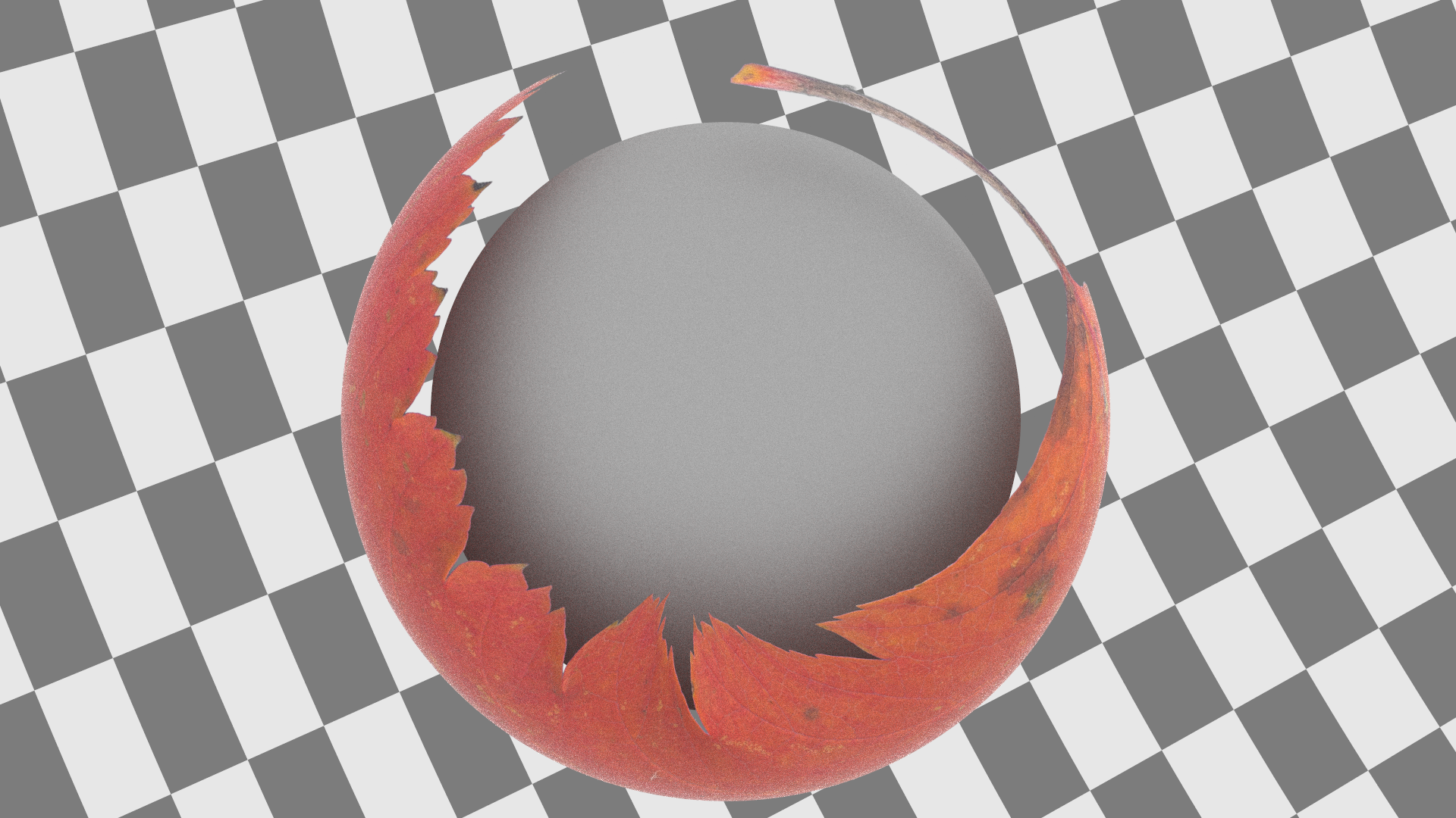
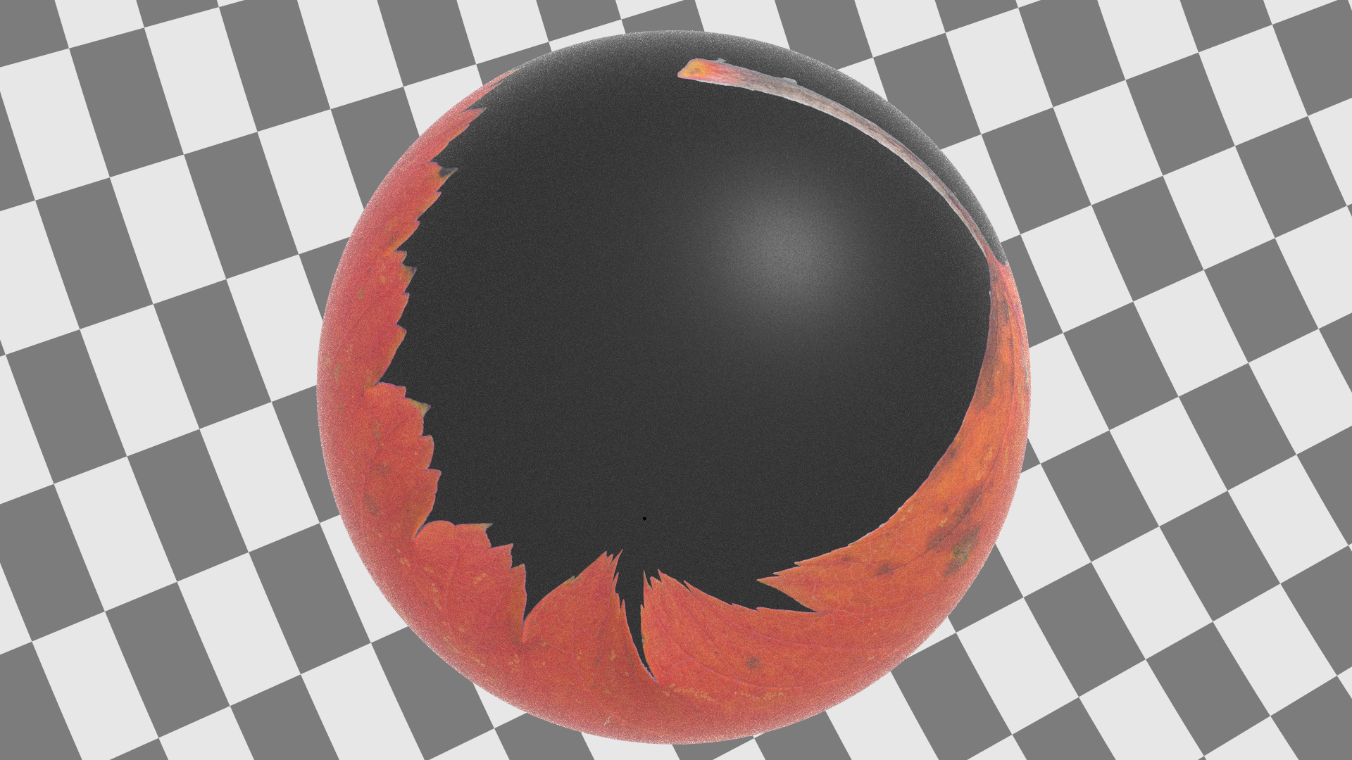
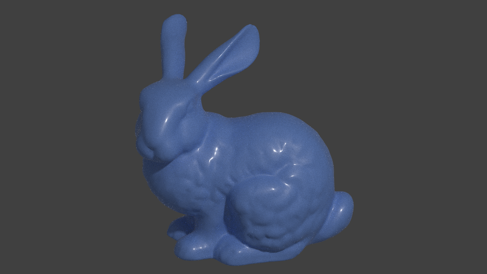
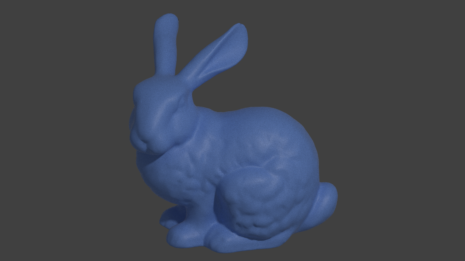
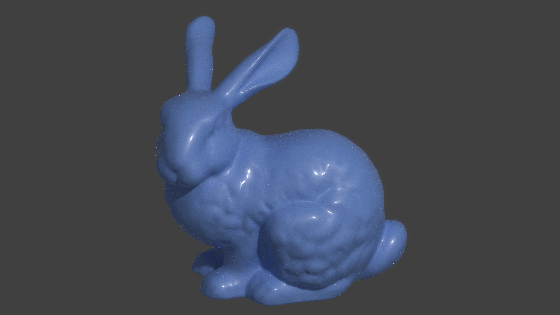
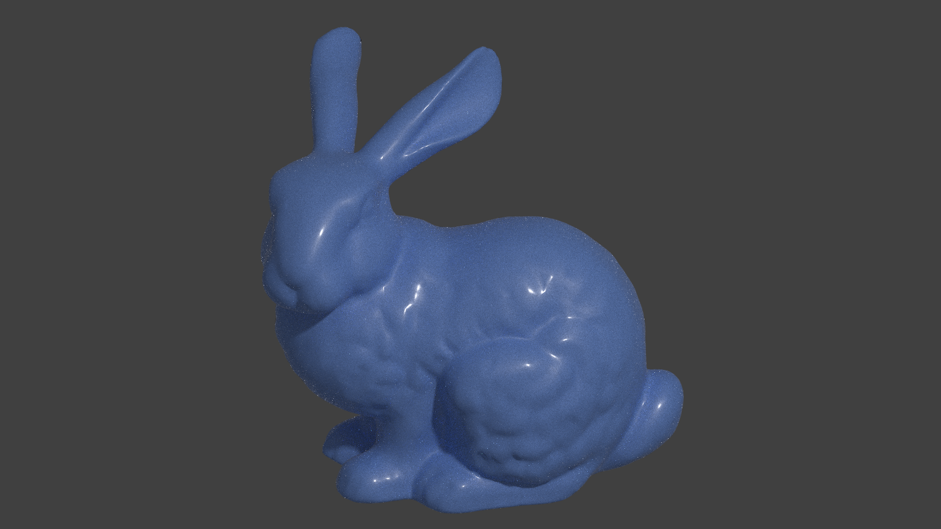
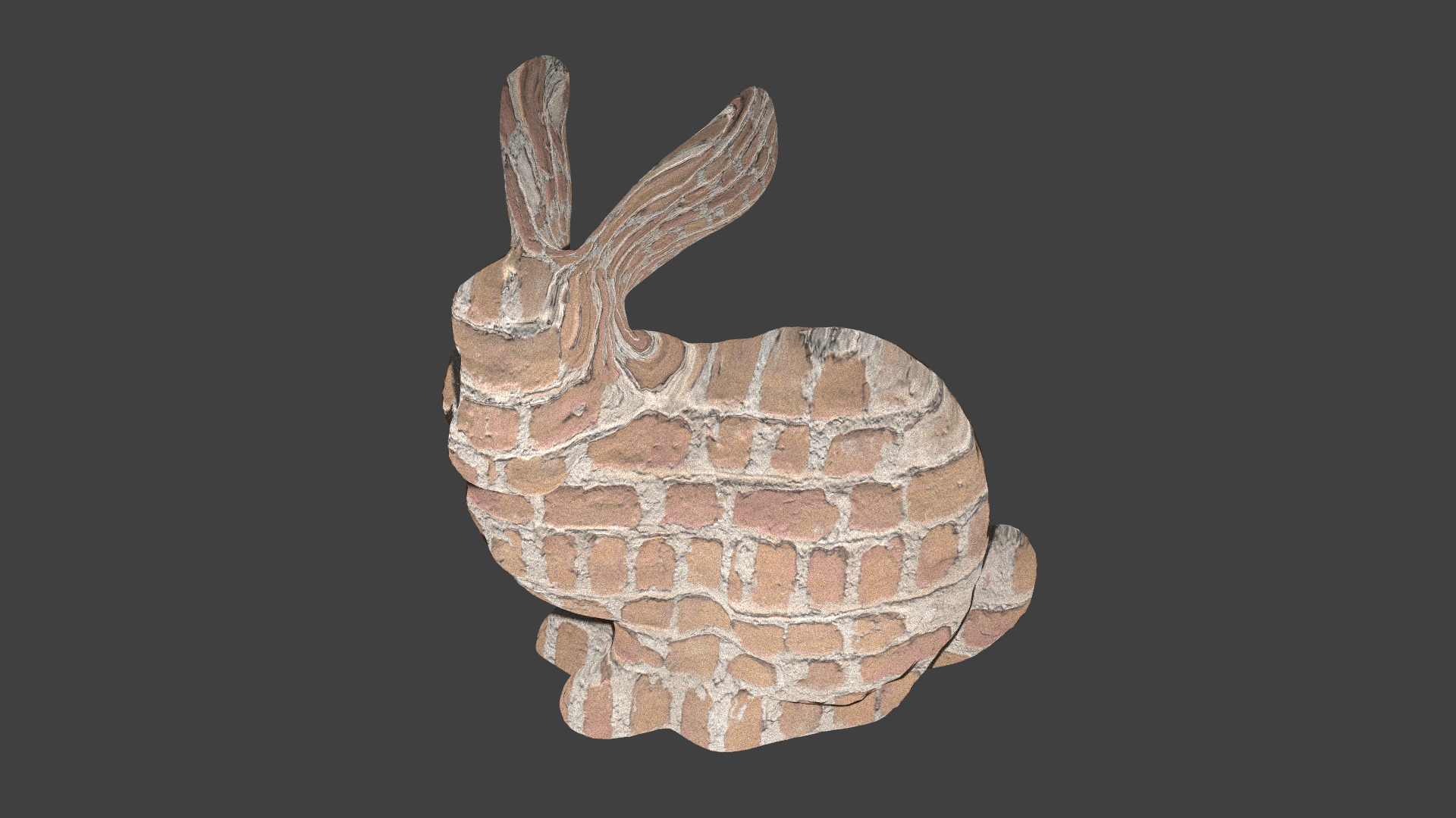
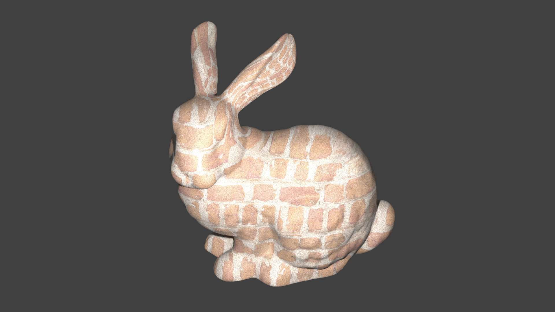
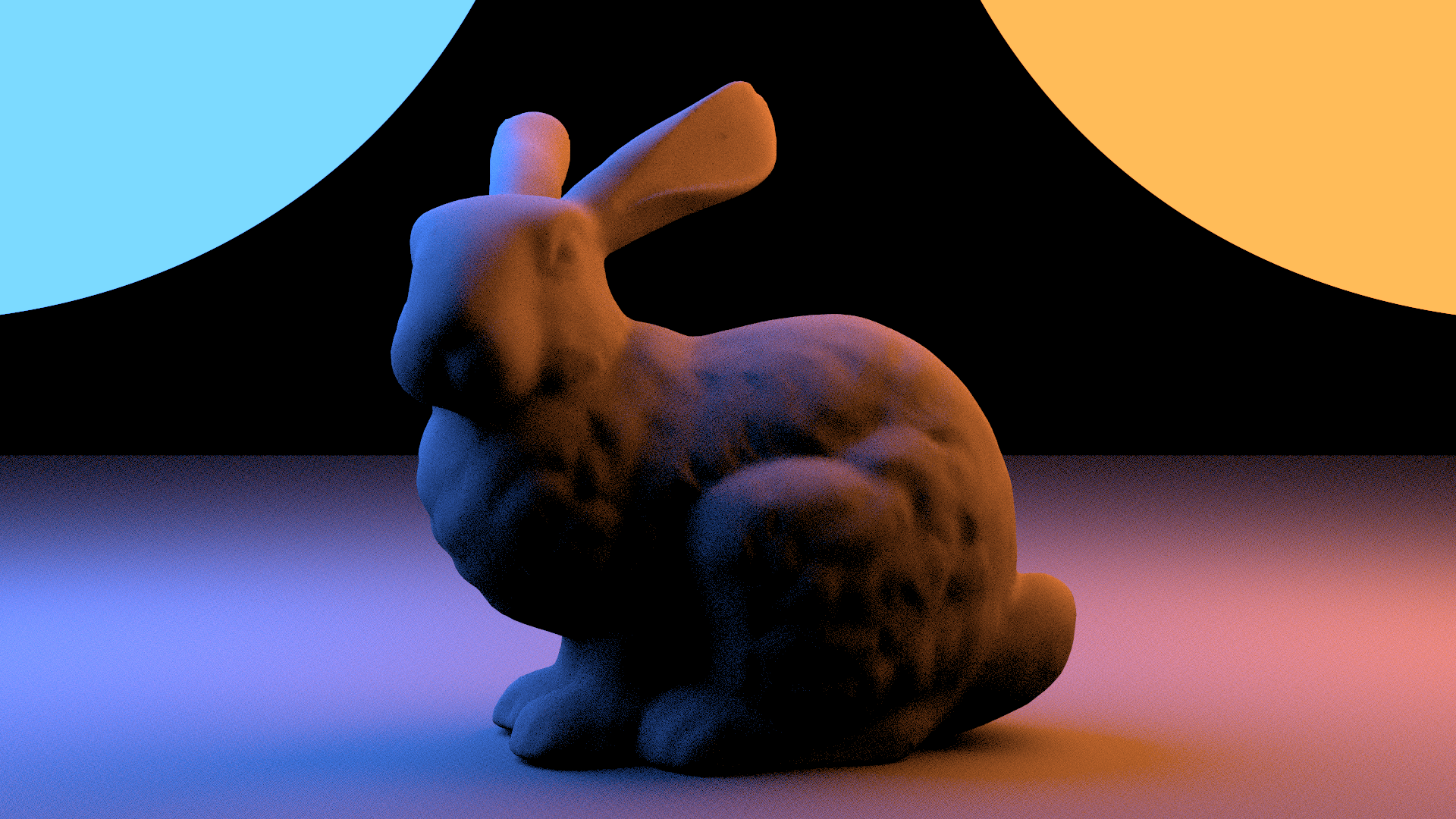
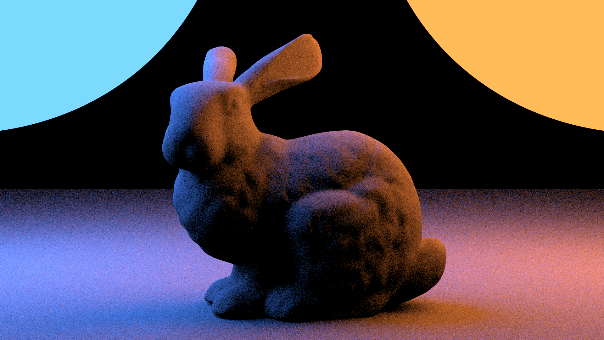
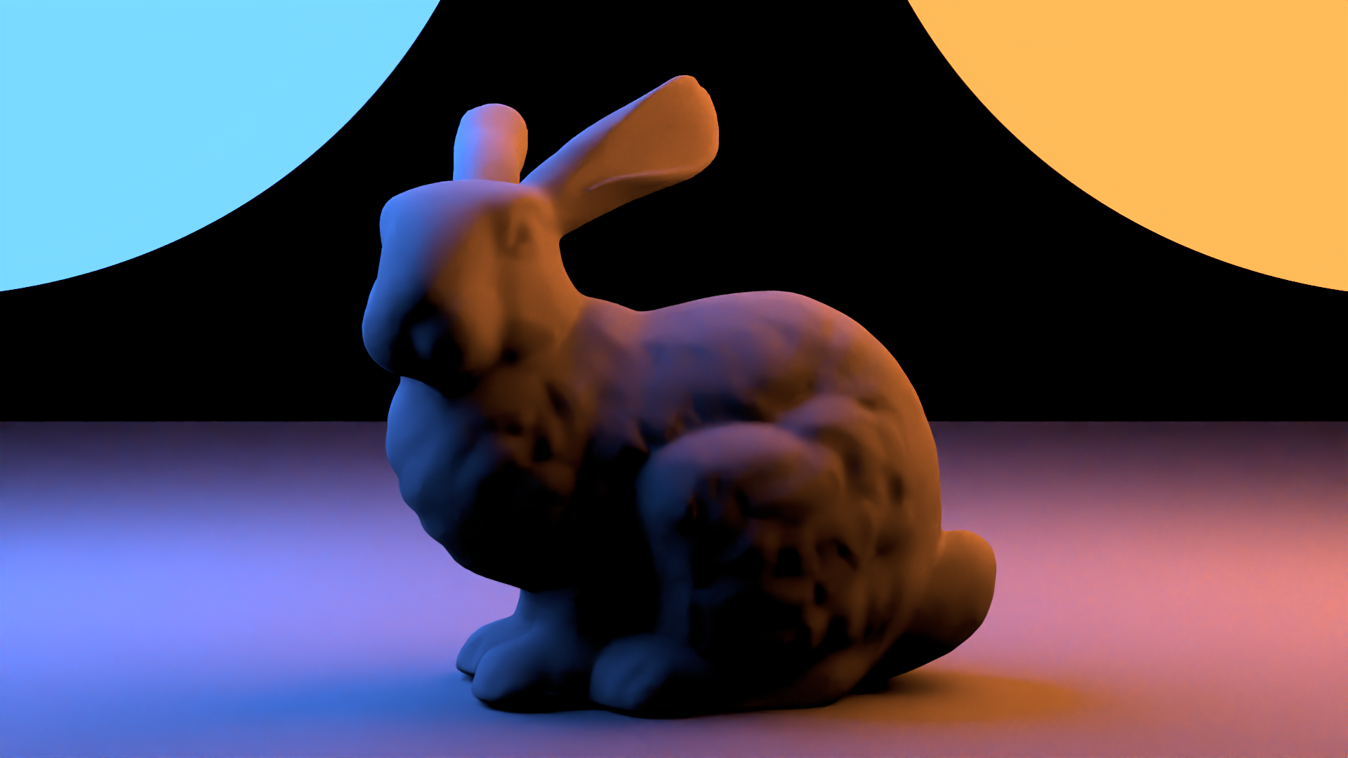
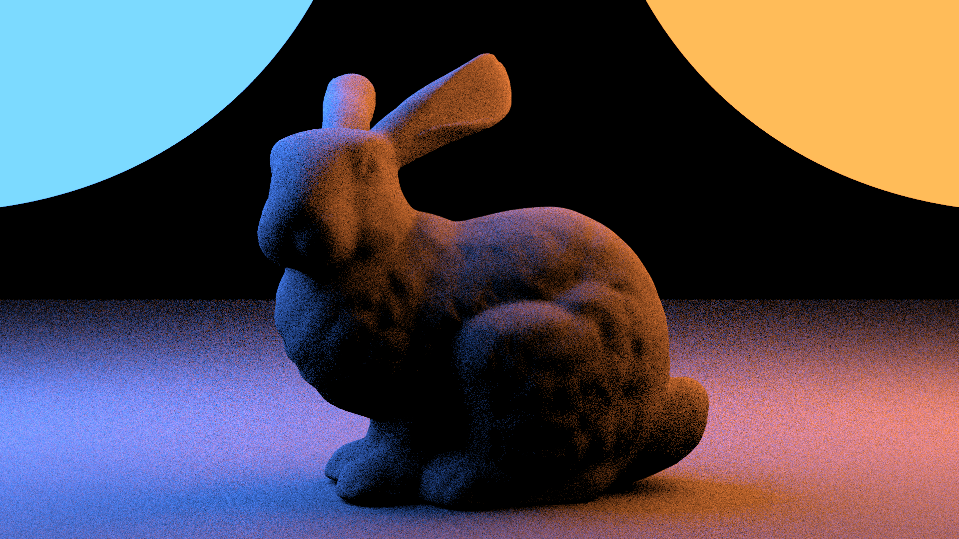
Drag slider to compare: Without Alpha Masking
(Left) vs With Alpha Masking (Right)
Description
Alpha masking is a powerful and efficient technique used
in computer graphics to create complex, highly detailed
organic surfaces without the computational cost of
modeling every single geometric detail. Instead of
constructing every individual leaf, twig, or intricate
cutout as a separate 3D mesh, we utilize a 2D texture
map where the alpha channel explicitly defines the
transparency of the object. By mapping transparency to a
texture, we can simulate intricate structures using
simple proxy geometry.
Implementation
We implemented this feature within the
Instance class by adding an optional
m_alpha texture property. The core logic
was added to the intersection routine (specifically in
intersectSceneWithAlpha). Instead of a
simple binary cutoff, we implemented
stochastic alpha masking. When a ray intersects
the geometry, the renderer samples the alpha texture at
the specific UV coordinate. This opacity value is
compared against a uniform random number (generated by
the sampler); if the random number is greater than the
alpha value, the intersection is probabilistically
discarded, allowing the ray to pass through as if
hitting empty space. This approach correctly
approximates partial transparency when averaged over
multiple samples.
See:
include/lightwave/instance.hpp
src/core/instance.cpp
Challenges
The primary challenge was integrating the masking logic
cleanly with the existing transformation hierarchy. We
had to ensure that the alpha test was applied
consistently whether the instance was transformed
(requiring ray transformation to local space) or
untransformed. Additionally, correct state management
was crucial: if an intersection is masked out, the
Intersection data structure must be
strictly reverted to its previous state (using
its = previousIts) to ensure the ray tracer
continues to search for valid hits behind the
transparent surface.
2. Clearcoat Material
Drag slider to compare: Standard Material (Left) vs
Clearcoat Material (Right)
Description
Standard materials often assume a single layer of
interaction, but real-world surfaces like car paint,
varnished wood, or glazed ceramic typically feature a
secondary layer: a transparent, reflective coating over
a base substrate. To simulate this, we added a
Clearcoat lobe to our Principled BSDF. This
feature adds a separate, glossy dielectric layer on top
of the existing diffuse and metallic layers. This
dual-layer approach allows us to render materials that
have both a rich underlying color and a sharp, distinct
specular highlight, significantly increasing the realism
of manufactured and coated surfaces in our scenes.
Implementation
We implemented the clearcoat as a distinct struct,
ClearcoatLobe, within the
Principled BSDF class.
BRDF Model: Unlike the metallic lobe which
uses GGX, the clearcoat follows the Disney
Principled BRDF specification by using the
GTR1 (Generalized Trowbridge-Reitz)
distribution (also known as Berry) for the
microfacet distribution. This creates the specific
"tail" falloff characteristic of clearcoats.
Masking/Shadowing & Fresnel: We utilized a
fixed alpha (roughness) of 0.25 for the Smith G1
geometry term and a standard dielectric Fresnel
approximation (Schlick) with R0 = 0.04
(representing common polyurethane or acrylic
coatings).
Sampling: The
Principled::sample method was updated
to probabilistically select between the diffuse,
metallic, and clearcoat lobes based on their
respective albedos. If the clearcoat is selected, we
sample the GTR1 distribution to generate a
reflection direction.
See:
src/bsdfs/principled.cpp
Challenges
The toughest challenge was correctly balancing the
energy conservation and probability weights when
combining three different lobes (Diffuse, Metallic, and
Clearcoat). Initially, adding the clearcoat energy
simply on top of the others led to overly bright
materials. We had to ensure the
combine function correctly calculated
selection probabilities based on the luminance of each
component, and that the Monte Carlo weights in
sample were properly divided by these
probabilities (e.g.,
sample.weight /= (1 - mettalicBoundary) for
the clearcoat) to maintain an unbiased estimator.
3. Post Processing (Bloom)
Drag slider to compare: Raw Render (Left) vs With
Bloom (Right)
Description
Bloom is a post-processing effect used to simulate the
optical phenomenon where very bright light overwhelms
the camera sensor (or the human eye), causing light to
bleed into the surrounding darker areas. While our path
tracer calculates physically accurate radiance, it
cannot natively simulate this lens artifact. By
implementing Bloom, we add a soft, glowing halo around
bright light sources—such as the sun, lamps, or emissive
geometry—significantly enhancing the perceived
brightness and dynamic range of the final image.
Implementation
We implemented the feature in the
Bloom class (subclassing
Postprocess) and a helper
GaussianFilter class. The process consists
of three main stages:
Thresholding: We first extract a "bright
pass" image by iterating over the input. Only pixels
with a luminance value exceeding a user-defined
m_threshold are kept; others are set to
black.
Gaussian Blurring: To create the soft glow,
we perform a Gaussian blur on the thresholded image.
We implemented a separable Gaussian filter.
Instead of performing an expensive 2D convolution
O(r2), we perform two 1D passes
(horizontal then vertical), reducing complexity to
O(r). To achieve a wide, smooth falloff, we apply
this blur iteratively, where each iteration blurs
the result of the previous one.
Compositing: Finally, we compute a weighted
sum of these blurred layers and add them back onto
the original input image, scaled by an intensity
factor to control the strength of the glow.
See:
src/postprocesses/bloom.cpp
Challenges
The main challenge was achieving a high-quality,
wide-radius blur without killing performance. A naive
implementation of a large Gaussian kernel is
computationally prohibitive (checking neighbors in a
massive N x N grid for every pixel). Implementing the
separable filter optimization was essential to
make the render time acceptable. Additionally, handling
image boundaries during convolution required careful
logic (using std::clamp) to ensure the blur
didn't introduce artifacts or crash at the edges of the
image.
4. Normal Mapping
Drag slider to compare: Without Normal Mapping
(Left) vs With Normal Mapping (Right)
Description
Normal mapping is a texturing technique used to simulate
high-frequency geometric detail—such as bumps,
scratches, or grooves—without increasing the polygon
count of the mesh. Instead of relying solely on the
interpolated vertex normals of the geometry, we sample
an additional 2D texture that encodes surface normal
vectors. These detailed normals are used for lighting
calculations (shading), creating the illusion of depth
and complexity on otherwise flat surfaces.
Implementation
We integrated normal mapping directly into the
Instance class, allowing any shape to be
enhanced.
Texture Property: We added an optional
m_normal texture member to the class.
Transform Logic: The core logic resides in
Instance::transformFrame. Before
transforming the intersection frame from object
space to world space, we check if a normal map
exists.
Mapping: If present, we evaluate the texture
at the intersection's UV coordinates. Since texture
colors are stored in the range [0, 1], we remap them
to the vector range [-1, 1] by an affine
transformation.
Application: We replace the intersection's
object-space shadingNormal with this
sampled vector and recompute the tangent using
Frame(normal).tangent to ensure the
shading frame remains orthogonal. Finally, the
standard instance transformation matrix is applied
to convert this new frame to world space.
See:
include/lightwave/instance.hpp
src/core/instance.cpp
Challenges
The main challenge was determining the correct order of
operations within the transformation pipeline. It was
crucial to apply the normal map modification
in object space (before applying
m_transform) rather than in world space. If
applied after the world transform, the normals from the
texture would not rotate or scale correctly with the
object. Additionally, ensuring that the tangent vector
was re-orthogonalized
(Frame(normal).tangent) after modifying the
normal was necessary to prevent degenerate shading
frames.
5. Low Discrepancy Sampling
Drag slider to compare: Random Sampling (Left) vs
Halton Sampling (Right)
Description
Standard pseudo-random number generators (independent
samplers) often produce "clumping" and large gaps in the
sample space, leading to noise that converges slowly. To
improve this, we implemented a Halton Sampler.
This is a low-discrepancy (quasi-random) sequence
generator that deterministically distributes sample
points to cover the N-dimensional domain more evenly
than random chance. By ensuring a well-stratified
distribution of samples, we significantly reduce visual
noise and aliasing artifacts for the same number of
samples per pixel, particularly in high-dimensional
integration tasks like path tracing.
Implementation
We implemented the Halton class inheriting
from Sampler. The core mechanism generates
samples using the radical inverse function
Φb(i), where b is a prime number base.
Dimension Mapping: We map each dimension of
the rendering equation (pixel X, pixel Y, lens U,
lens V, etc.) to a specific prime base (2, 3, 5, 7,
...). The first two dimensions (Base-2 and Base-3)
are reserved for image space positions to ensure
good spatial stratification.
Index Computation: A crucial part of the
implementation was the
seed(pixel, sampleIndex) function.
Unlike a simple global counter, we compute a
specific global Halton index for every pixel to
ensure that samples land exactly within that pixel's
boundaries. This required solving the Chinese
Remainder Theorem to find an index i such that
Φ2(i) ≈ x and
Φ3(i) ≈ y.
Randomization: To prevent visual artifacts
(structured patterns) common with raw Halton
sequences, we added support for
randomization strategies:
Digit Permutation (scrambling the digits of
the radical inverse expansion) and
Owen Scrambling.
See:
src/samplers/halton.hpp
src/samplers/halton.cpp
src/samplers/utilities/lowdiscrepancy.hpp
src/samplers/utilities/lowdiscrepancy.cpp
src/samplers/utilities/permutation.hpp
src/samplers/utilities/permutation.cpp
src/samplers/utilities/primes.hpp
Challenges
The most complex aspect was implementing the global
index mapping for the seed function. We had
to calculate multiplicative inverses and extended GCDs
to solve the system of congruences required to "jump"
the generator to the correct sequence index for a
specific pixel (x, y). Without this math, the sampler
would generate valid Halton points globally across the
unit square, but they wouldn't necessarily align with
the specific pixel being rendered, breaking the
stratification benefit.
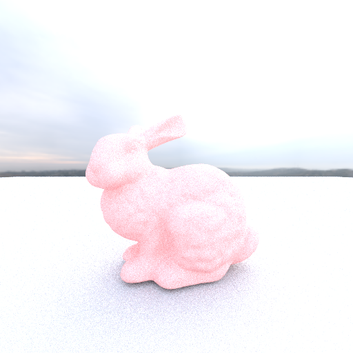
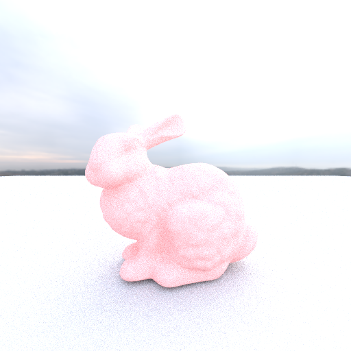
6. Image Denoising
Drag slider to compare: Noisy Output (Left) vs
Denoised Output (Right)
Description
Monte Carlo path tracing is notorious for producing
grainy, noisy images when the sample count is low.
Increasing the sample count to resolve this noise can
increase render times linearly or worse. To combat this,
we integrated Intel® Open Image Denoise (OIDN), a
high-performance, AI-based library capable of
reconstructing clean images from noisy inputs. This
allows us to achieve high-quality results with
significantly fewer samples per pixel, drastically
reducing overall render time.
Implementation
We created a new Denoise class inheriting
from Postprocess. The implementation
involves:
Device Abstraction: The implementation
initializes an OIDN device (supporting CPU, CUDA,
Metal, etc.) based on user configuration, ensuring
hardware acceleration is used where available.
Auxiliary Buffers (AOVs): To improve the
denoiser's ability to distinguish between geometry
edges and noise, we feed it auxiliary feature
buffers. Specifically, we support optional
albedo and normal maps.
Data Transformation: Before passing data to
OIDN, we preprocess the normal maps. Our renderer
outputs normals in the [0, 1] color range, but OIDN
expects vector data in [-1, 1]. We transformed the
normals in an affine manner to remap these values
correctly.
Execution: The execute method
transfers the input image (and optional AOVs) to
OIDN-managed buffers, runs the "RT" (ray tracing)
filter with HDR mode enabled, and reads the cleaned
result back into the output image.
See:
src/postprocesses/denoise.cpp
Challenges
The primary challenge was ensuring the correct format
and range of the auxiliary data. OIDN is sensitive to
the quality of input features; feeding it incorrect
normal vectors (e.g., in the wrong coordinate space or
range) leads to worse artifacts than not using them at
all. We had to implement a specific check where normal
maps are only used if albedo maps are also present, as
OIDN's documentation suggests normals are less effective
in isolation. Additionally, managing the memory transfer
between the host application and OIDN device buffers
required careful handling to support different backend
types (like Metal or CUDA) robustly.
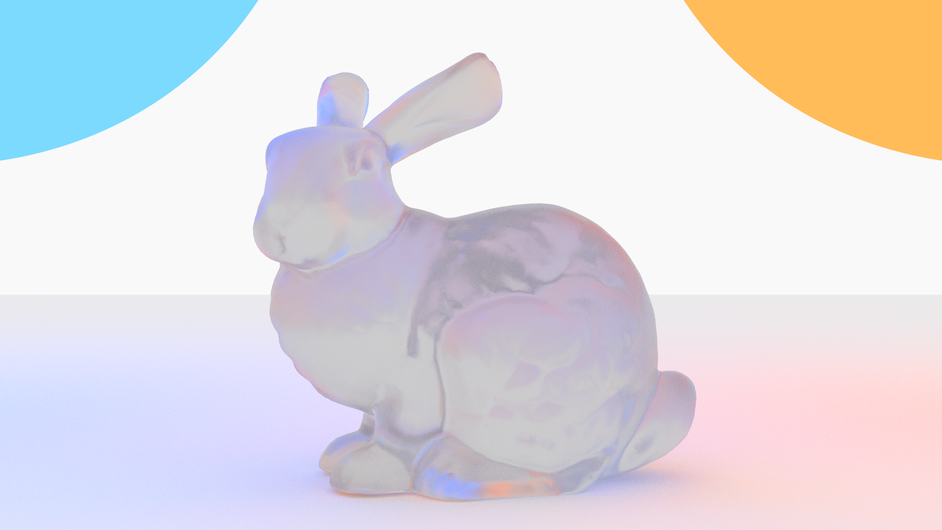
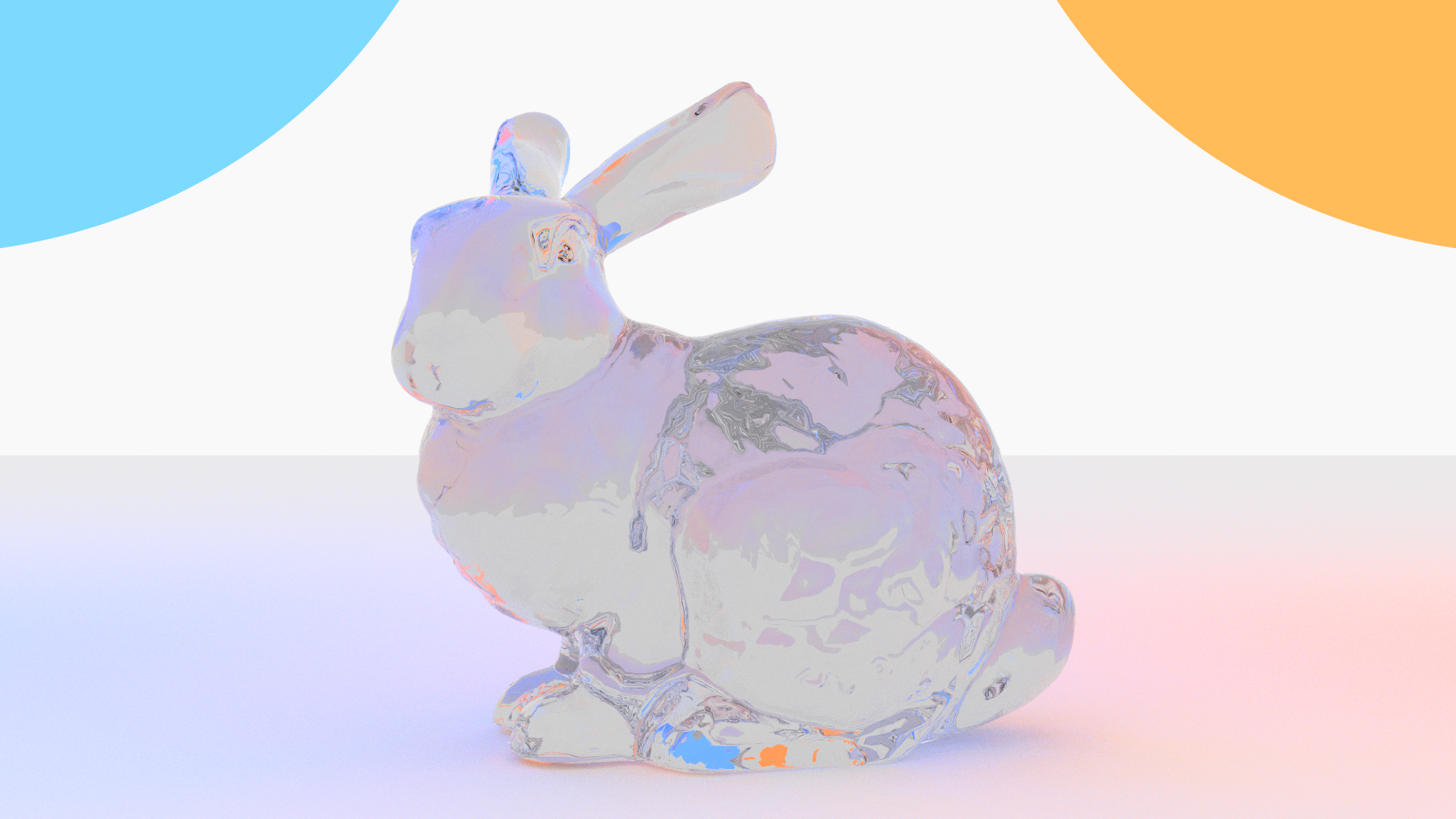
7. Rough Dielectric
Drag slider to compare: Perfect Dielectric (Left)
vs Rough Dielectric (Right)
Description
Standard dielectrics (like clear glass or water) assume
a perfectly smooth surface. However, many real-world
transparent materials, such as frosted glass, ice, or
etched crystal, possess microscopic surface
irregularities that scatter light. To simulate this, we
implemented a Rough Dielectric BSDF. This model
combines the physics of refraction with microfacet
theory. Instead of a single, sharp refraction direction,
light rays are scattered according to a statistical
distribution of micro-surface normals, creating blurry
refractions and softened specular highlights.
Implementation
We implemented the RoughDielectric class,
which unifies logic from both rough conductors and
smooth dielectrics.
Microfacet Distribution: We use the GGX
distribution to model the surface roughness. The
roughness parameter (α) is derived from the
square of the texture value: α =
roughness2.
Sampling: In sample, we first sample a
microfacet normal ωh using the
Visible Normal Distribution Function (VNDF). We then
calculate the Fresnel term F for this microfacet.
Based on the ratio of reflected to transmitted
luminance (weighted by F), we stochastically decide
whether to reflect or refract the incoming ray
relative to ωh.
Evaluation: The
evaluate function handles both
reflection (same hemisphere) and refraction
(opposite hemisphere).
For reflection, it behaves similarly
to a rough conductor but uses the dielectric
Fresnel term.
For refraction, it uses the
generalized microfacet equation for
transmission. Crucially, the half-vector for
refraction is defined as ωh
= -η ωi +
ωo.
See:
src/bsdfs/roughdielectric.cpp
Challenges
The most difficult part of this implementation was
correctly handling the
change of variables (Jacobian) in the refraction
term. Unlike reflection, where the solid angle change is
straightforward, refraction compresses or expands the
solid angle based on the ratio of indices of refraction
(-η). Failing to include the determinant of the
Jacobian results in incorrect energy levels (dark
glass). Additionally, ensuring that the half-vector
ωh always points into the simpler
medium (or consistently handling the sign of
ωh) was essential to avoid NaN values
during the Fresnel calculation.
8. Env Sampling
Drag slider to compare: Standard Sampling (Left) vs
Importance Sampling (Right)
Description
Environment maps (HDRI) are excellent for providing
realistic, complex lighting from "infinity." However,
naive sampling strategies treat every pixel on the
environment map as equally important. In scenes with
high-contrast lighting—like a bright sun in a dark
sky—uniformly sampling the sphere means we rarely hit
the sun, resulting in excessive noise and slow
convergence. To fix this, we attempted to implement
Importance Sampling for the environment map. This
technique constructs a probability distribution based on
the brightness of the texture, ensuring that we cast
significantly more shadow rays toward bright areas
(light sources) than dark ones.
Implementation
We modified the EnvironmentMap class to
support Next Event Estimation (NEE) driven by texture
intensity, attempting to follow the implementation
details found in
Physically Based Rendering (PBRT).
Precomputation: In
computeDistribution, we compute the
luminance of the texture and build a
Distribution2D structure (utilizing a
marginal and conditional CDF) to allow picking UV
coordinates proportional to their brightness.
Sampling: In sampleDirect, we
utilize this distribution to sample a UV coordinate
(u, v) and a corresponding probability density p(u,
v).
Mapping: We convert the sampled UVs to
spherical coordinates (φ = 2πu, θ =
π v) and finally to a local direction vector.
Weighting: We calculate the Monte Carlo
weight using the inverse of the PDF. We included the
Jacobian determinant for the equirectangular
projection (2π2 sinθ) to convert
the PDF from image space to solid angle space.
See:
src/lights/envmap.cpp
src/lights/utilities/distribution.hpp
src/lights/utilities/distribution.cpp
Challenges & Current Status
The current implementation is buggy. Despite
correctly building the 2D distribution function and
sampling coordinates according to the CDF following the
PBRT reference, the resulting lighting is incorrect. The
output image with and without the importance sampling
seems to be the same.The main challenge lies in the
complex chain of coordinate transformations and PDF
conversions (Image Space to Spherical Coordinates to
Solid Angle). Somewhere in the interplay between the
Jacobian term (sinθ), the normalization factors,
and the texture coordinate mapping, errors were
introduced that we have not yet resolved.
9. Area Light
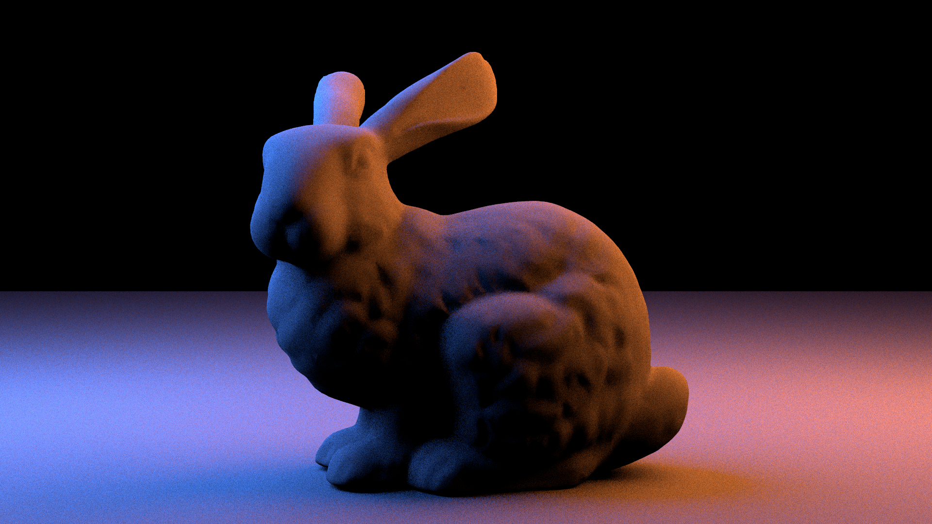
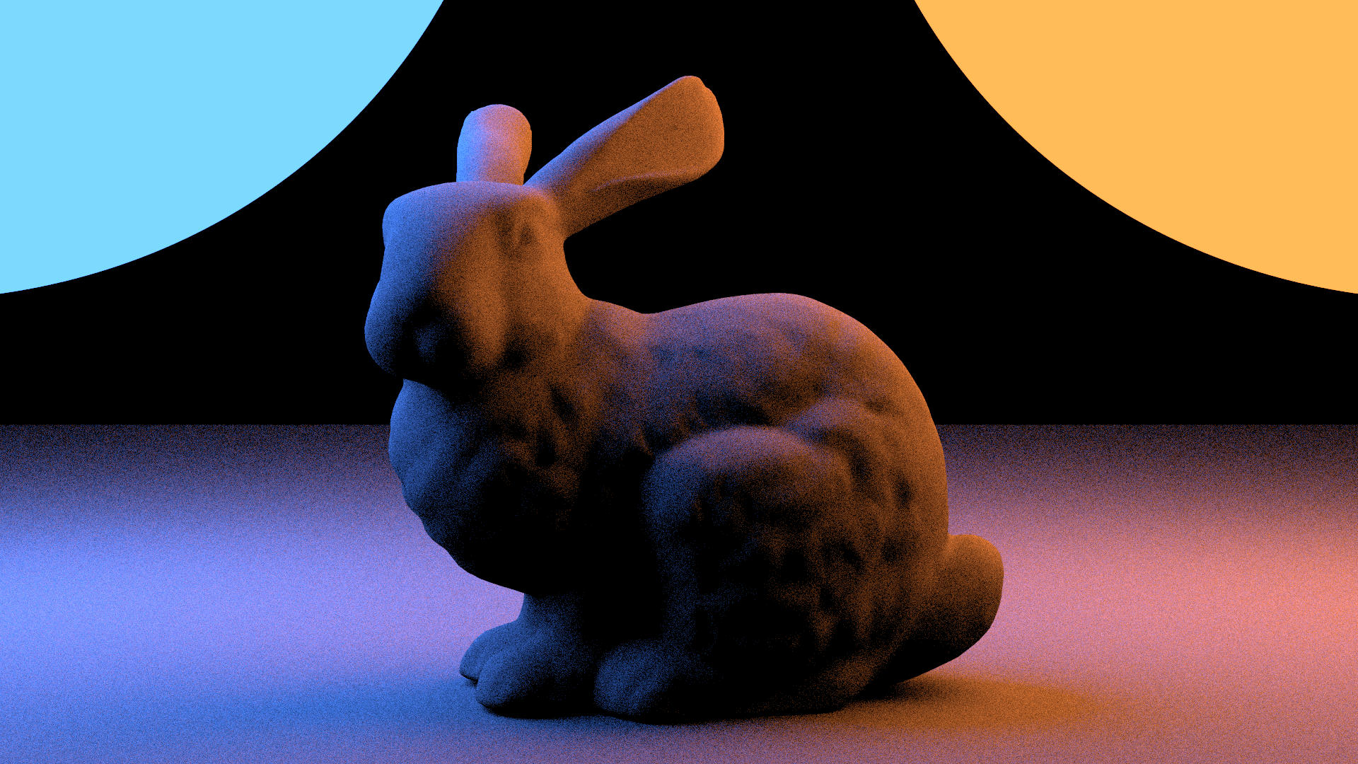
Drag slider to compare: Point Light (Left) vs Area
Light (Right)
Description
Relying on random chance to hit small, bright light
sources (like light bulbs or the sun) results in
extremely noisy images, as most rays simply miss the
light. To resolve this, we implemented
Next Event Estimation (NEE) for emissive shapes.
Instead of waiting for a path to accidentally hit a
light source, we explicitly sample points on the surface
of area lights at every shading point. This technique,
known as direct light sampling, drastically reduces
variance and noise by ensuring that the contribution of
light sources is calculated consistently.
Implementation
We implemented a new AreaLight class that
wraps an Instance (which contains the
geometric shape and emission profile).
Sampling Geometry: The core logic relies on
the Instance::sampleArea method (and
the underlying Shape::sampleArea),
which selects a point on the surface of the shape.
Conversion to Solid Angle: The sampling
occurs in area measure (finding a point p on
the surface with probability density pA).
However, the rendering equation integrates over
solid angle. In sampleDirect, we
perform the necessary change of variables
considering the angle between the light's normal and
the incoming ray, and the distance between the
shading point and the light.
Emission Evaluation: Once a point is sampled,
we query the Emission component of the
instance to get the radiance Le.
Challenges
The main challenge was ensuring the correct geometric
relationships between the shading point and the sampled
light point. Specifically, handling the
geometry term G(x, y) correctly is vital. If the
distance squared term (d2) or the cosine
foreshortening at the light source (cosθ) is
omitted or incorrect, the lighting intensity falls off
incorrectly with distance or angle. Additionally, we had
to ensure robust handling of edge cases, such as when
the sampled point is extremely close to the origin
(causing division by zero) or when the probability
density (PDF) is zero.
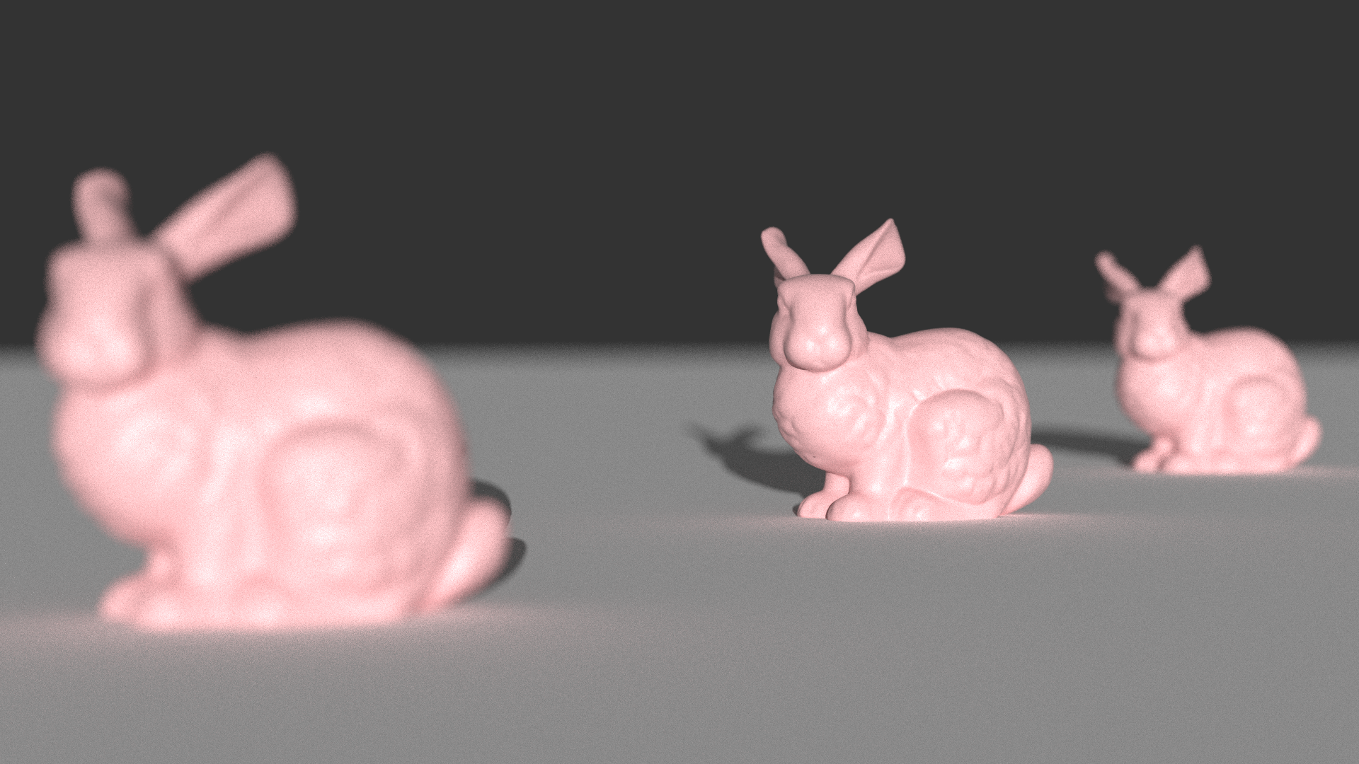
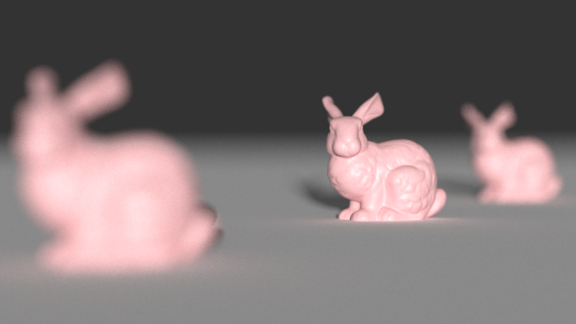
10. ThinLens
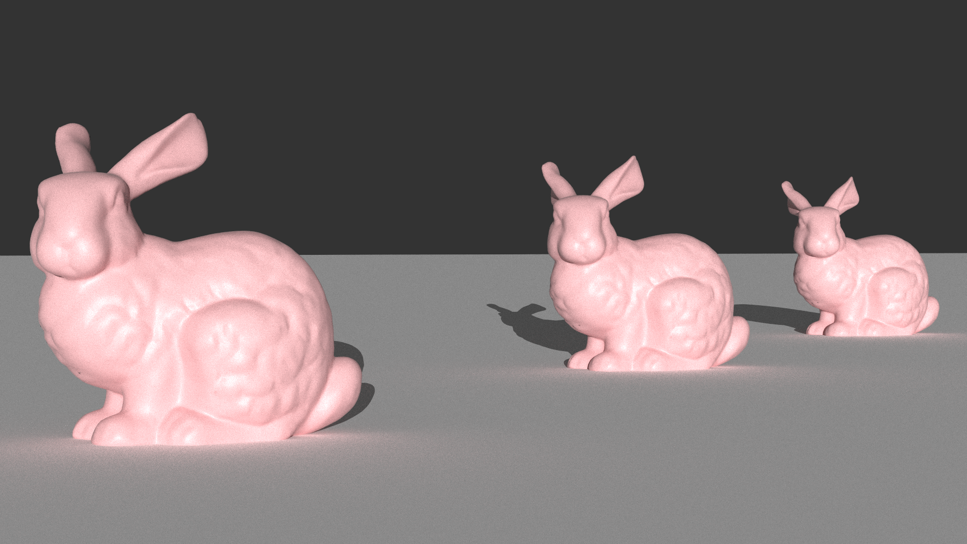
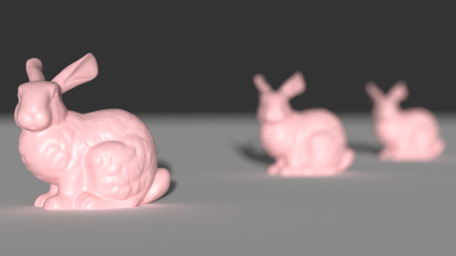
Perspective Camera
Low Focal Distance
Mid Focal Distance
High Lens Radius
Description
Standard computer graphics cameras usually follow the
"pinhole" model, where the aperture is infinitesimally
small, resulting in an image that is perfectly sharp at
all distances. Real cameras, however, have a finite
aperture size, which causes objects outside the focal
plane to appear blurry—an effect known as depth of
field. To simulate this optical phenomenon, we
implemented a Thin Lens camera model. By defining
a lens radius and a focal distance, we can control which
parts of the scene are in focus and the intensity of the
background/foreground blur (bokeh).
Implementation
We modified the Perspective camera class to
support finite apertures.
Focal Plane Calculation: In the
sample
method, we first calculate where a ray from a
standard pinhole camera would intersect the plane of
focus. This is determined by the
m_focalDistance.
Lens Sampling: Instead of starting every ray
at the origin (0,0,0), we sample a random point on
the surface of the lens. We use concentric disk
sampling
(squareToUniformDiskConcentric) to map
uniform random numbers to a disk of radius
m_lensRadius.
Ray Generation: The final camera ray is
constructed by connecting the sampled point on the
lens to the target point on the focal plane. This
ensures that all rays originating from the lens
converge at the focal distance (keeping that plane
sharp) while diverging elsewhere (creating blur).
Challenges
The main challenge was correctly establishing the
geometric relationship between the screen space sample,
the lens sample, and the focal plane. We had to ensure
that the initial direction vector was scaled correctly
so that it strictly intersected the focal plane at the
focal distance. If this intersection point is calculated
incorrectly, the plane of focus shifts unpredictably,
making it difficult to focus on specific objects in the
scene. Additionally, ensuring that the sampling was
uniform over the lens disk (using concentric mapping)
was important to avoid "clumping" of rays that would
bias the shape of the bokeh.