This feature is conceptually quite simple. We want to allow light rays to pass through certain shapes, without modifying the geometry. This allows us to render objects like leaves and broken windows that are otherwise just simple rectangular meshes. To do this, we need a texture or channel that encodes the transparency of each point on the mesh (using texture coordinates).

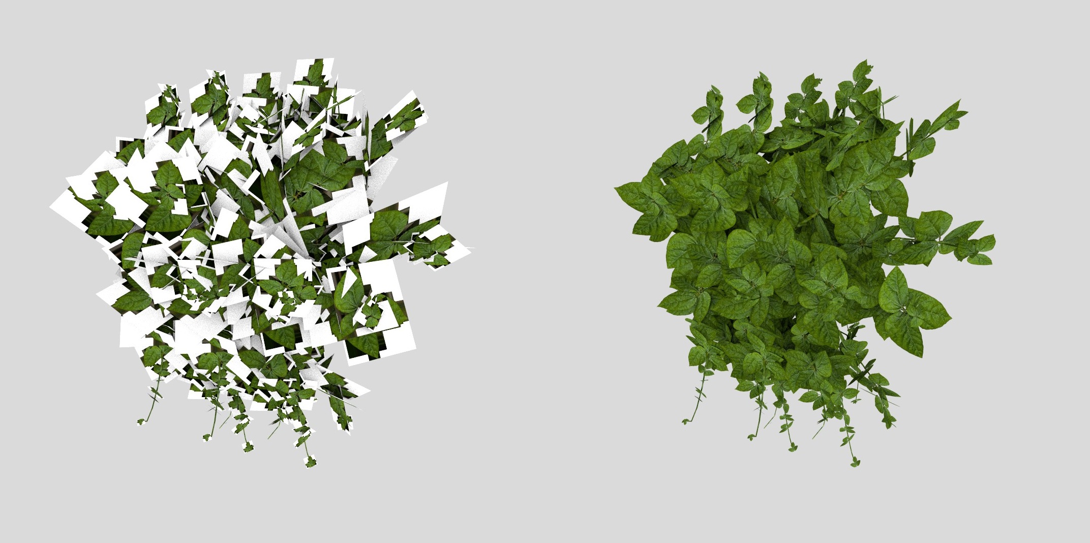
In order to implement this feature, we need to introduce an alpha masking function to the instance.cpp file, which queries the alpha texture information from the XML file. We then call this function in the intersect() and transmittance() functions. It's important to implement this function here as it will be able to affect all intersections from one central location. We can modify the instance class to hold an alpha texture.

After shooting a ray and determining that it does intersect the object, we call the alphaMasking() function. Inside, we check the transparency of the intersected point. If a point has a transparency of 0, then a light can pass through it, making it look transparent (non-intersectable). If a point has transparency 1, then it's solid, and we thus have an intersection. If it is in between the two, we intersect it with a probability equal to the transparency. If we passed through the point, we are not done yet however. The ray may not intersect other parts of the mesh. So we set our previous intersection point as the new origin, and shoot a ray in the same direction, and then repeat the above procedure for each intersected point, until we have a valid intersection, or the ray leaves the object entirely.

Challenges

• The texture object only stores the first 3 channels, r, g, and b. So instead of using the PNG's built in alpha channel, I instead had to introduce a new tag in the XML file that contains a greyscale alpha masking texture.
• One bug only became apparent when rendering two overlapping alpha-masked objects: the texture of one object would leak into the next. As it turns out, the intersect() function keeps track of the previous intersection's t value and restores it if there isn't a new intersection. However, when doing alpha masking, even if there isn't an intersection, the intersection object nonetheless is overridden (since an intersection can happen but is discarded). So we need to keep track of the entire previous intersection object and restore it, not just the t value.

The spotlight feature introduces a new light type, similar to point lights, but constrained to a cone whose dimensions can be set by the user. Like point lights, the spotlight is not intersectable; it can only be sampled during next event estimation. The light also radiates along a sphere, similar to point lights, though in the case of spotlights, the surface area along the sphere is restricted along the cone of the spotlight.

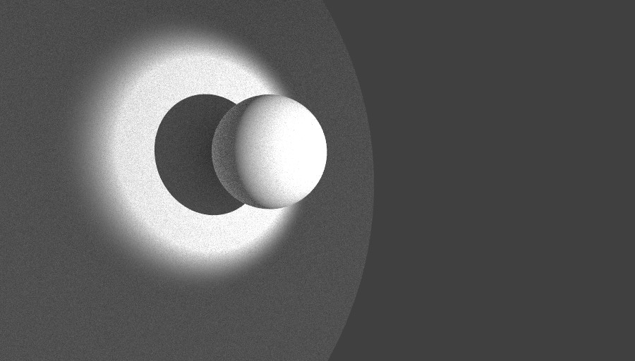
In order to implement a spotlight, we need to query the power, transform, inner angle, and outer angle of the spotlight. The inner angle gives us the cone of light where the power is as its maximum, while the outer angle gives us the angle at which the light fades away completely. In between these two angles, the light needs to smoothly subside as to not create a sharp edge between the lit and unlit areas.

For my implementation, I only needed to add one new file: src\lights\spot.cpp. This file contains a function, falloff(), which calculates how much the light subsides based on the angle of the light ray, following the scheme found in PBRT. There is also a function that calculates the area along which the light radiates. We then use both of these functions to calculate the light weight, which is otherwise similar to point lights.

Challenges

• As mentioned, instead of radiating in a full sphere, the light radiates within a cone. Calculating the area of the sphere inside said cone was conceptually at least, challenging. I was unsure of whether to use the inner or outer angle.

We already have emissive objects in our renderer, which can be randomly sampled during pathtracing, and their contributions are counted as emissions. However, this can make the scene look very noisy. A better approach is to instead sample them during Next Event Estimation. This makes the object more likely to be sampled, and thus, reduces the noise. Now, an area light is by definition intersectable, so if we were to have the same object be both an area light, and an emissive object that can be intersected normally during path tracing, we run the risk of double counting the light contribution. As such, we will also need to implement Multiple Importance Sampling to ensure that doesn't happen (if we want to use both).

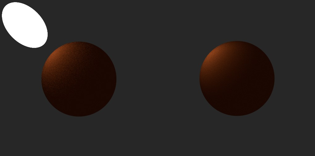
Querying Area lights information is simple. We just need to wrap an emissive shape in an area light tag. We can then define a file src\lights\area.cpp where we query any information we need. Note that any shape that is considered an area light needs to have implemented the sampleArea() function, allowing us to sample the area

In the sampleDirect() function of the AreaLight class, we can use the sampleArea() function to get the pdf, and convert it from local to global space. Afterwards, we can convert it to the solid angles formulation, and use it to compute the power of the area light along the chosen sample.
In order to convert to global coordinates, I just assumed I had a small rectangular patch where my sampled point was, and calculated the scaling factor of said patch as its area approached zero. Since the patch's area can be calculated as u × v, we can apply the transform to u and v individually, and then shuffle the terms around until we have the world space area written explicitly in terms of the local area. This will involve a scaling factor that depends on the transformation itself, as well as normal at the sampled point.
To convert to solid angles, we need to satisfy the equation P(ω) dω = P(A) dA, relating the PDF per unit angle with the PDF per unit area. Since dA = (length² / cos(θ)) dω, we can convert between the two using: P(ω) = P(A)(cos(θ) / length²) ,

Multiple Importance Sampling requires the probability of hitting an area light in Next Event Estimation, and the probability of hitting the light during path tracing. We use these in order to calculate the weight used to scale the NEE contribution and Le contributions in order to ensure no double counting. I had to modify both the BsdfEval and DirectLightSample structs such that they both carry the PDF of sampling a point on them. I then went back and set this parameter for all of our existing lights and BSDFs. The probability of sampling a point on a light during Next Event Estimation is the PDF multiplied by the probability of choosing this light source. The probability of sampling the point in the path tracer is just the PDF (evaluated not at the point being sampled, but the previous point receiving the contribution).

Challenges

• In the AreaSample we get from our shape, we have access to a PDF, which is the probability of picking a point on the surface. However, this value is in local coordinates, and in the area formulation. We need it in global coordinates and in the solid angle formulation. As such, I had to convert the area PDF to world space and then convert it to solid angles, or vice versa. I struggled in deciding whether doing the transformation in either order would offer up any benefits.
• For MIS, we have to multiply both Li (NEE) and Le by a weight. But first, we need to determine if the contribution needs to be weighted. For NEE, we needed to ensure that the light we were intersecting was also visible to the path tracer (not just an area light, but an emissive surface as well). For the path tracing sample, we needed to ensure that the shape we intersected was also an area light. The latter was simple, but the former was more complicated, and I still haven't found a way to do it.

Bloom is a post process that essentially radiates light from very bright areas into their immediate surroundings, making the image look more realistic.

In order to implement this, I defined a new post process subclass in a file called src\postprocesses\bloom.cpp. To start, the object queries the lightThreshold, sigma, and passes parameters from the XML file.

In an image or array, we then store only the pixels whose luminance exceeds the threshold, and keep all other pixels black. Then, using a Gaussian kernel with a radius equal to sigma, we convolve the image, that is, we average out the values that the kernel covers. This is what allows the light to bleed out into surrounding areas. We can then repeat the blurring process according to the number of passes we have, and add the convolved image back to the original.

Instead of using a two dimensional Gaussian kernel, it's both faster and easier to apply the one dimensional Gaussian kernel on both directions separately. By decoupling the variables, and implementing the convolution in two separate 1D passes and storing the results, we can reduce the time complexity from quadratic to linear for each pixel in the texture. The convolution K * u applies the following operation on the image:

We can start with the integral:

We can discretize this in two dimensions, where x and y refer to the current pixel, and i and j are the pixels being looped over while convolving:

The kernel K is Gaussian (written here without the σ for clarity), and can be expressed as:

This in turn can be decoupled:

And then decoupled for efficiency:

If we were to compute the inner sum first and store it:

We can reuse it for the outer sum, without having to recompute anything:

This allows us to apply the one dimensional Gaussian kernel twice, at the cost of having to store the intermediate values.

Challenges

• Overall, this wasn't a difficult feature to implement, though I have worked a bit with convolutions in other courses. The aspect that I struggled with the most the first time around however, was the decoupling of the variables.

So far, we've only used geometric and shading normals. Both are expected to have been calculated using the object's geometry. Normal mapping on the other hand gives us a third option, and the ability to use normals that visually modify the object surface without actually modifying the geometry. This in turn allows us to have a perfectly smooth, simple mesh, while also having crevices, fissures, and bumps appear when rendered. This can be done by simply using a texture to encode new normal values at each point on the object.

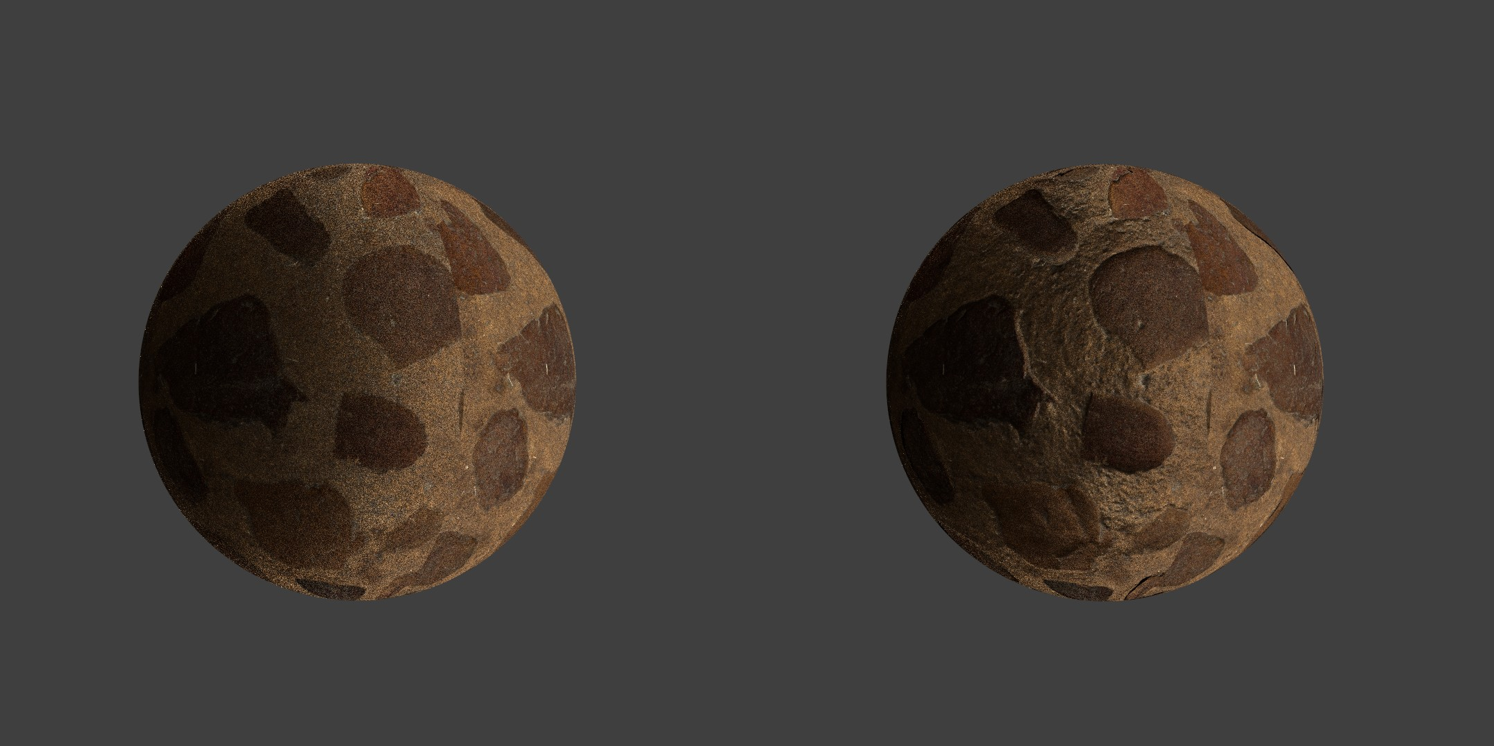
In order to implement this, can simply query the normal texture from the XML file. We can modify the instance class to hold a normal texture. Like alpha-masking, we can define a normalMapping() function in the instance.cpp file, since this is where all intersections will take place. The normals are encoded in the texture as colors, and they are stored in tangent space (shading space). So, for each intersection, the normalMapping() function retrieves the normal for the point, and then transforms it to world coordinates using the shading frame of the intersection.

Challenges

• This was a very straightforward feature to implement. The only part I struggled with was deciding whether or not to modify the tangent once the normal was updated (ensuring it remains orthogonal to the new normal). In the end I decided against that, as the output looked correct regardless, though it's still not something I am entirely certain about.

The Thin Lens feature introduces a new camera type. It is similar to a perspective camera, but differs in that it blurs out-of-focus objects (those that are both too close and too far), mimicking how actual cameras work.

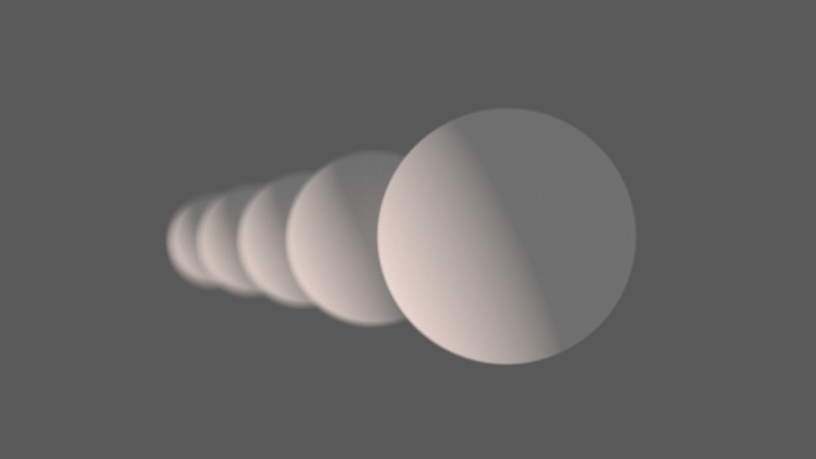
In order to implement this, I only needed to write one new file, src\cameras\thinLens.cpp. In this file, we can query the exact same parameters from the XML file as a perspective camera, along with two new ones: the lens radius, and the focus plane distance. The focus plane determines the distance at which objects need to be in order to be in focus. Objects farther or closer than that are blurred.

Thin lens camera rays need to focus on the focus plane, that is, the rays need to hit the same point as the perspective camera ray of light would have hit. So we can randomly sample a point on the lens, a nd connect it to the perspective camera ray intersection. Because it only matches the perspective camera for objects on the focus plane, only those objects will be in focus.

Challenges

• Overall, this was a simple feature to implement. PBRT is good reference, and it contains all needed information, leaving no room for ambiguities.

Sometimes, instead of a mesh or a parametrically defined geometric object, we have an implicit signed distance function f, such that the surface occurs at all points x where f(x) = 0. Such a shape can be intersected using Ray Marching. Signed Distance Functions in general are great for visualizing procedurally generated shapes, such as fractals. It does not need to store anything, except for the signed distance function.

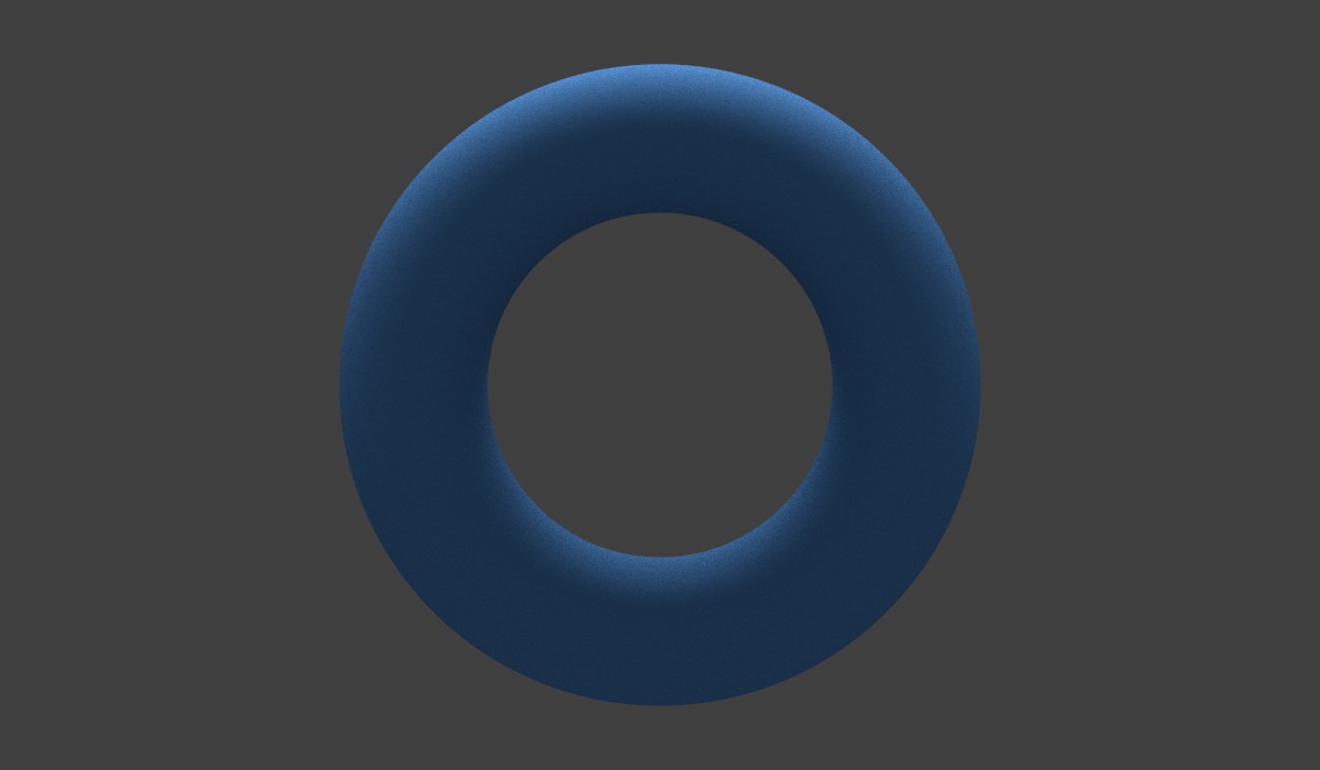
In my implementation, I used a Torus signed distance function, as it's a simple shape to model and verify, with a simple signed distance function. From the XML file, the only parameter to query is the ratio of the large and small radii of the torus. I only added one new file src\shapes\torusSDF.cpp, which includes a Torus subclass that extends the shape class.

In order to intersect a shape given by a signed distance function, we can use ray marching. Because the signed distance function gives us (possibly an approximation) of the distance to the object, we can simply evaluate it at the origin of the ray, and then march the absolute value of the distance along the ray. Because the distance function returns the shortest distance to the object, the amount we march along the ray is conservative, which means we are unlikely to pass through the object in one pass. We can then repeat this process, using a minimum step size in order to ensure we actually intersect the object in finite time. Since we have a signed distance function, we know we've intersected the object when the signs of the output changes.

To calculate the normal I used both an explicit torus normal formula, as well as a numerical approximation using central differences (to approximate the derivative at each point) which works for an arbitrary shape.

Challenges

• I am unsure of how to compute UV coordinates for arbitrary signed distance functions (for a torus specifically, it is simple). For normals, we can just use central differences, but I'm not sure if texture coordinates generalize as well.