Computer Graphics 2024
—
Team Abra

Team Members

Bao Huy Nguyen

Anh Dang Le Tran

Motivation

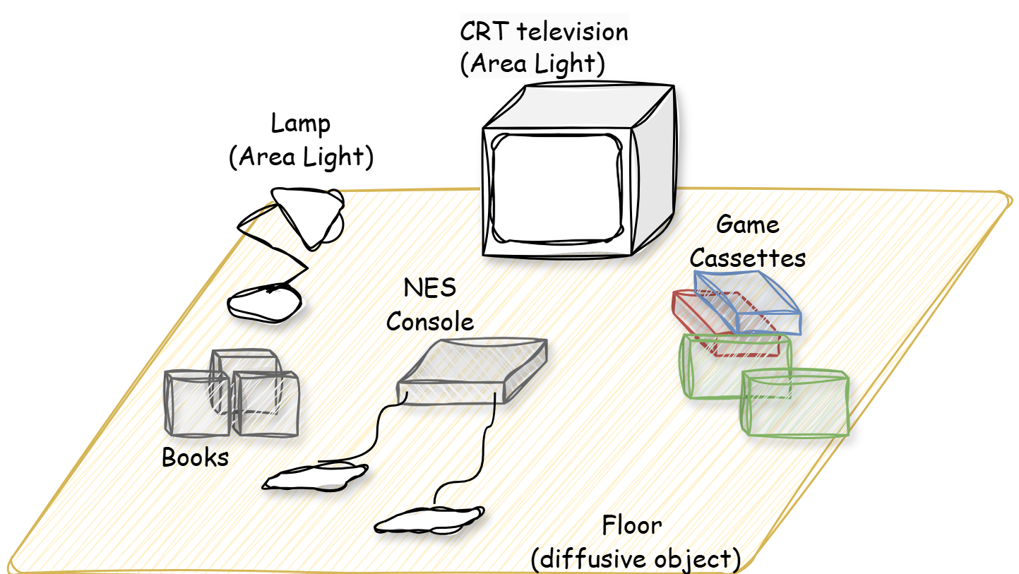
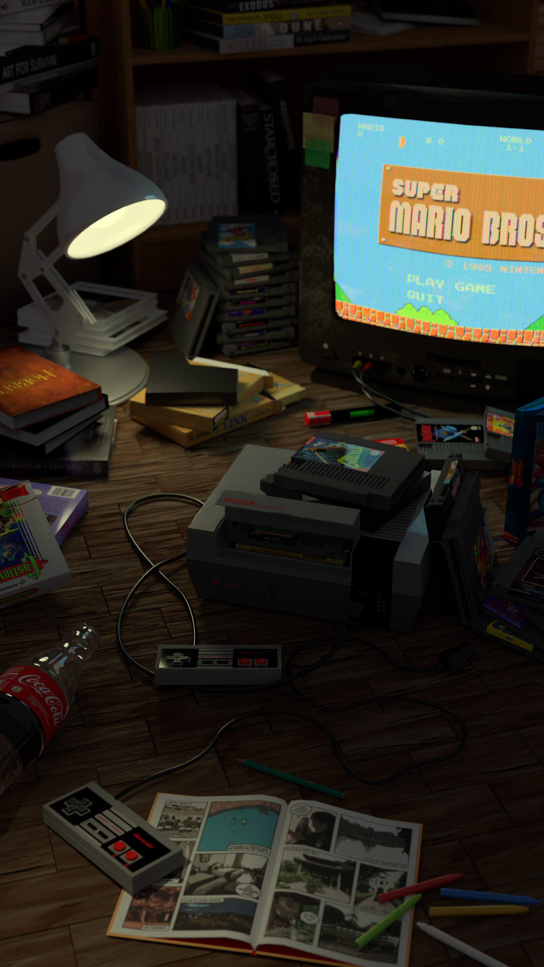
When I saw the topic, I quickly recalled to my working place. Messy, unorganized, chaostic sometimes dirty maybe are the words that other people would use to describe it. However, somehow, strangely, to me it’s still really “organised” since I know where things are in my desk (or somehow I purposely and unconsciously put them there), and they are there just because of balance and harmony.

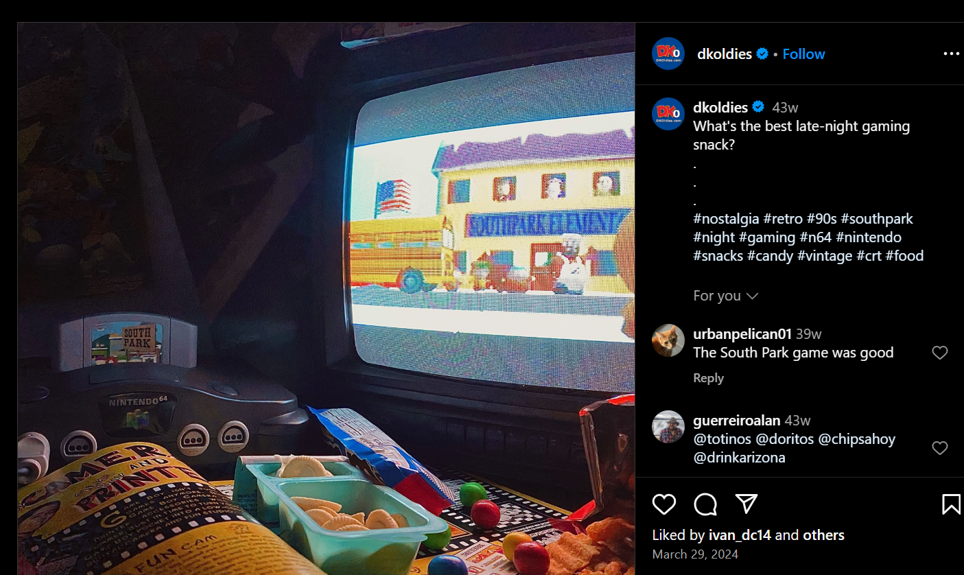
In addition, we are really interested in the nostalgia trend recently hence we want to model a scene that reminds everyone (maybe mostly boys) about their childhoods, video games in late night and no homework. Chilling time, peaceful moment in the messy place.

Simple Features

Shading Normals

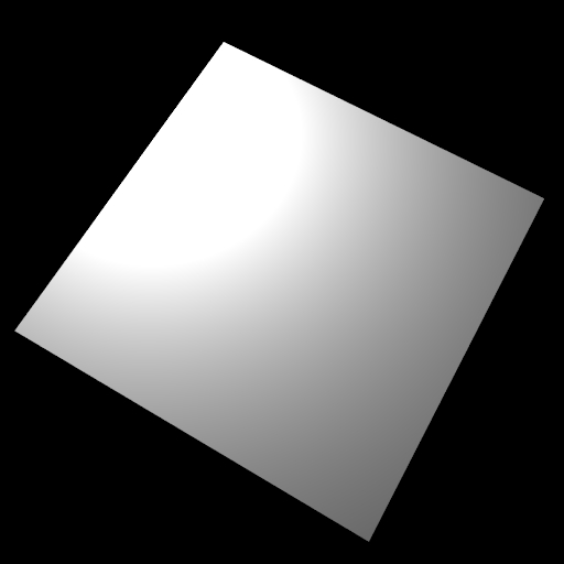
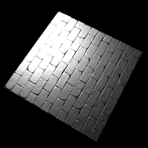
Shadding Normals/ Normal Mapping is a cheap and easiy way to add more details to a geometry without having to model a complex and detailed mesh. We employ this technique to render the highly detailed and complex objects like a wooden floor. To implement this, we include normal map texture property ref<Texture> m_normals in the class instance.hpp to get the normal texture if provided. Then we re-compute the tangent vector based on the new shading normal in Instance::transformFrame().

Code:

include\lightwave\instance.hpp
src\core\instance.cpp

Alpha Masking

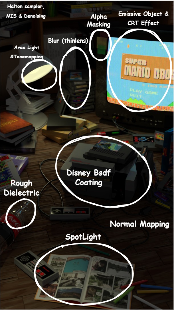
For our scene, we want to have several transparent sticker notes attached to the CRT television as decorations. These objects is not fully opaque and we can see other objects behind it. To this end, we implement alpha masking similar to shading normals above. The instance class will find the provided alpha texture in a xml file.

Code:

include\lightwave\instance.hpp
src\core\instance.cpp

Halton Sampler

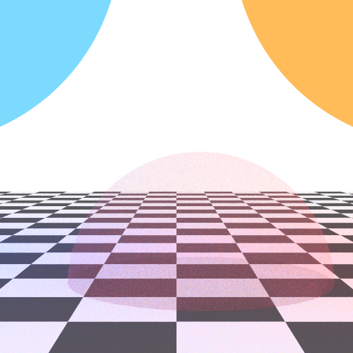
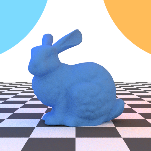
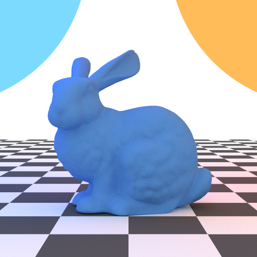
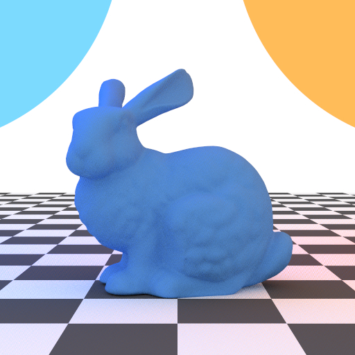
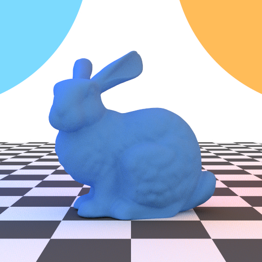
The Independent sampler sometimes, unluckly, produces many samples in a same region and that leads to high variant results. This may require a large number of sample to cover all the possible incoming light directions to an intersection point to achieve less variance. However, the more samples, the slower renderer is. To get better visual quality with the same amount of samples, we follow the intruction from PBR to implement Halton Sampler. The visual quality is significantly enhanced compared to Independent sampler with the same amount of samples per pixel.

Code:

src\samplers\halton.cpp
src\utils\lowdiscrepancy.hpp

Below are the results of using Independent Sampler and Halton sampler with 3 different randomizer strategies. All of them use same number of samples, 64.

Independent	Owen Scramble

Permute Digits	Radical Inverse

Post Processing

Tone Mapping

Reinhard

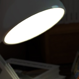
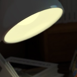
Although human visual perception has a relatively high dynamic range, most of monitors can only represent RGB color in range [0, 255] or [0, 1]. Output of our renderer is an high dynamic range image without an upper intensity limitation. To map a high dynamic range image to [0, 1] to display it, we refer this guidline to implement tonemapping alogrithms

Code:

src\postprocess\tonemapping.cpp
src\utils\imageprocessing.hpp

Image Denoising

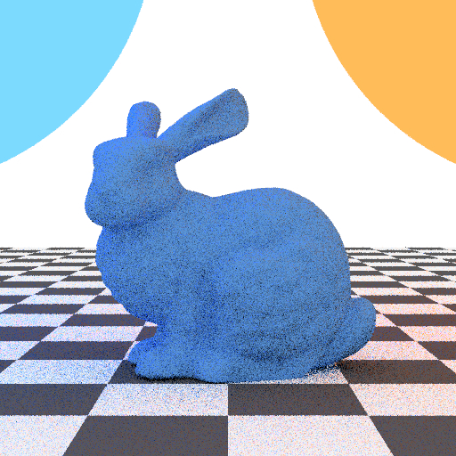
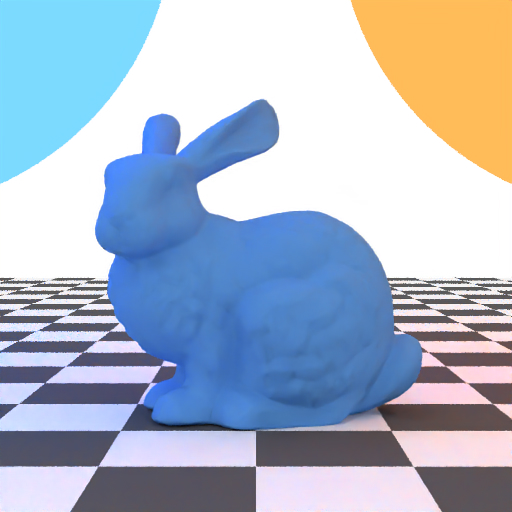
Since our render uses the Monte Carlo method to compute the high-dimensional integral in the rendering equation, a large of number of samples is required to achieve a visally appealing result, which presents a computational burden. Our scene has a considerable number of objects in which using a low number of samples would produce noisy results. To this end, we integrate Intel®Open Image Denoise library to our renderer to reduce noise of outputs.

Code:

src\postprocess\denoise.cpp

Rough Dielectric

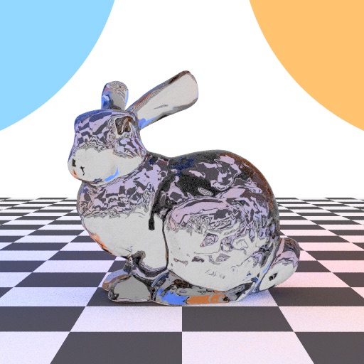
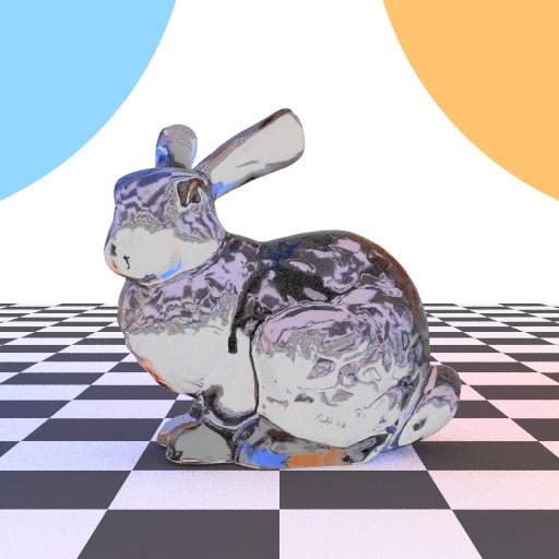
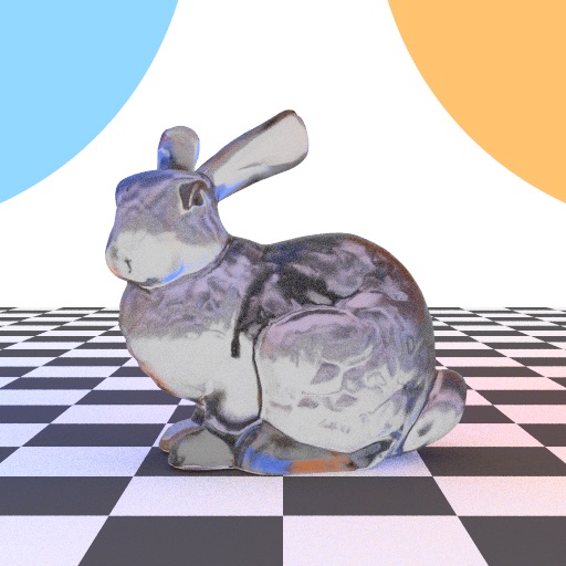
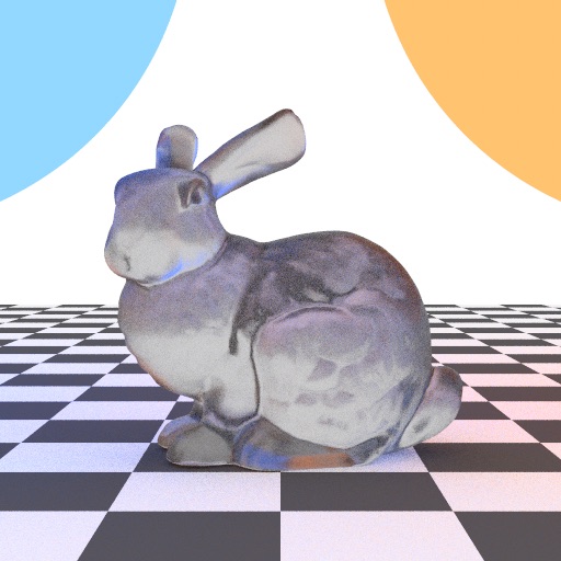
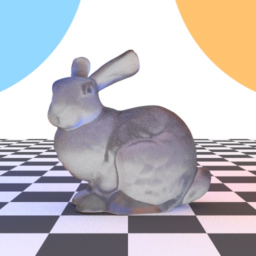
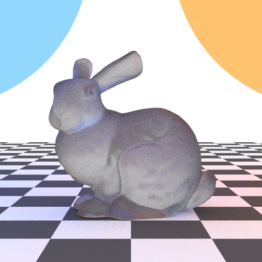
We want to increase a little bit of realism to our glass material, hence implement rough dielectric bsdf to add a little bit of roughness to our Coca-Cola bottle . We follow the Microfacet Models for Refraction to implement that bsdf class.

Code:

src\bsdfs\roughdielectric.cpp

roughness = 0.0	roughness = 0.1	roughness = 0.2
roughness = 0.3	roughness = 0.4	roughness = 0.5

Area Light

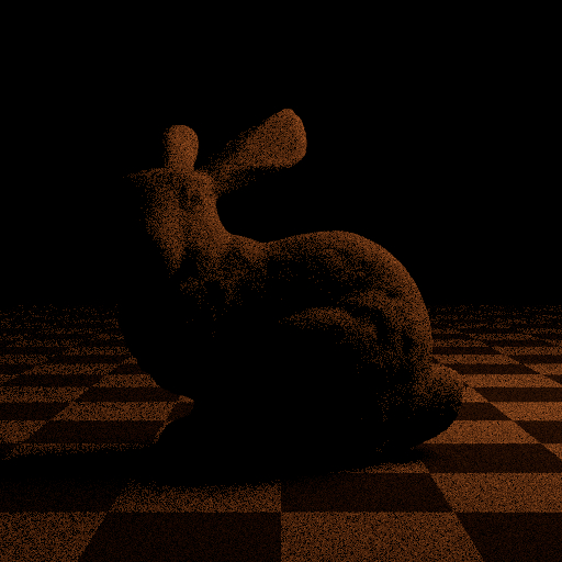
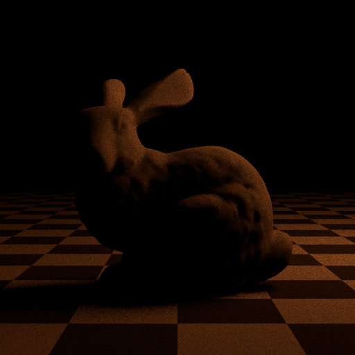
We implement area light class for the lamp' bulb and the screen of CRT television (which are natuarlly area lights).

Code:

src\lights\area.cpp
src\shapes\mesh.cpp
src\shapes\rectangle.cpp
src\shapes\sphere.cpp
include\lightwave\shape.hpp

Spot Light

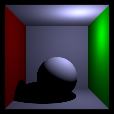
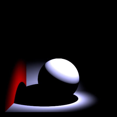
Our scene has the vibe of late game night and sometimes we only want to shine a specific area but not the whole sence. Point light and directional light are not a good choice in this case. To this end, we refer to PBR to implement another light class, spotlight, to handle this task.

Code:

src\lights\spot.cpp

Intermediate Features

Thinlens Camera

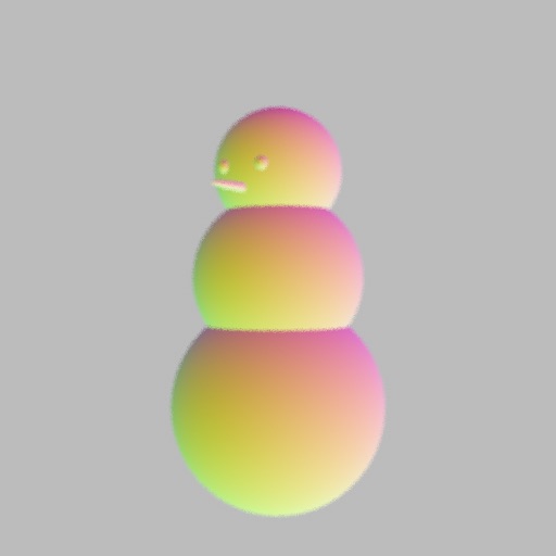
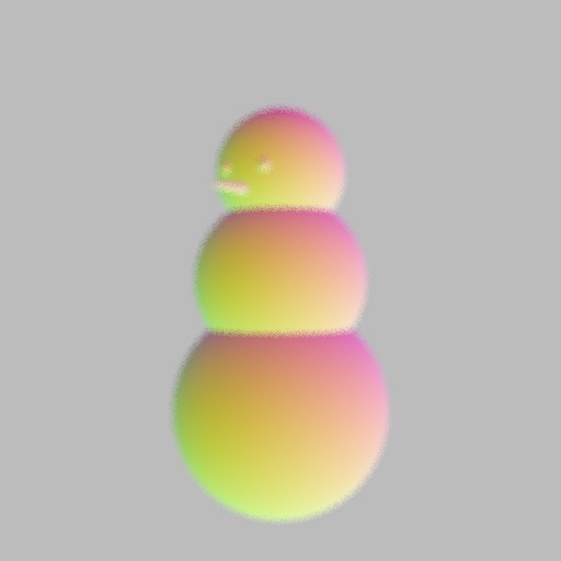
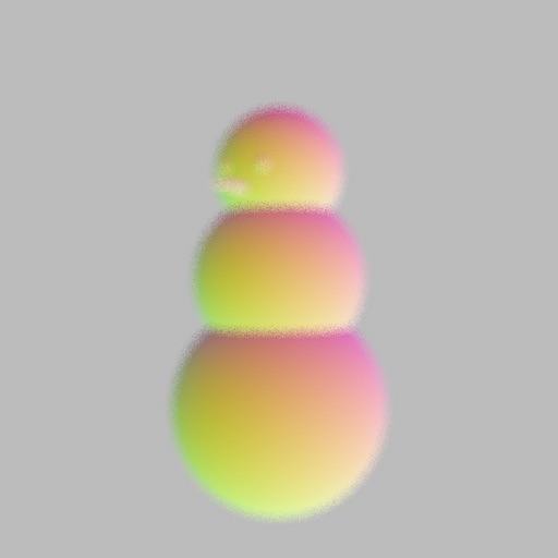
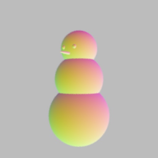
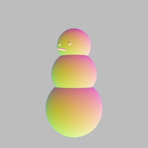
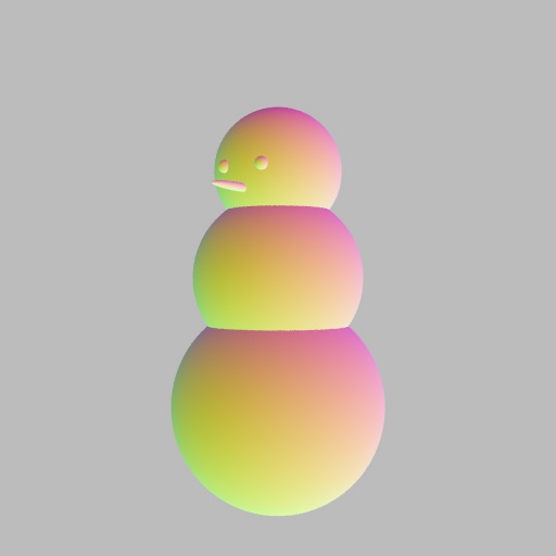
The perspective pin pole camera model in our renderer could not capture the focus effect like real life camera, which may reduce the realism. To simulate the depth of field effect of the real life cameras, we follow PBR to implement a thin lens camera model.

Code:

src\cameras\thinlens.cpp

MIS Path Tracer

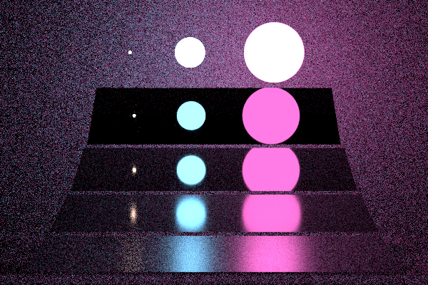
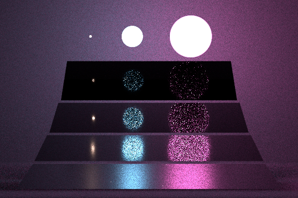
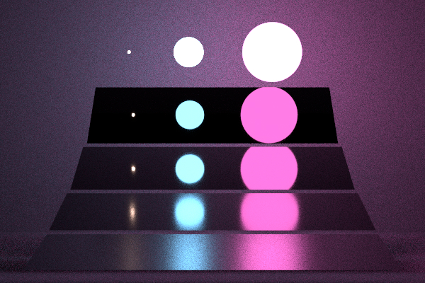
Faithfully tracing each ray in BSDF sampling will produce unbias results in rendering but requires a large number of samples and high depth to achieve those results. On the other hand NEE although significantly reduce noise by directly accounting direct illuminace from light source, will fail in case of smooth surfaces which requires idirect illumination. To balance both, we refer the video lecture by Prof. Ravi Ramamoorthi to implement MIS Path Tracer.

Code:

src\integrators\mis_pathtracer.cpp

Disney BSDF

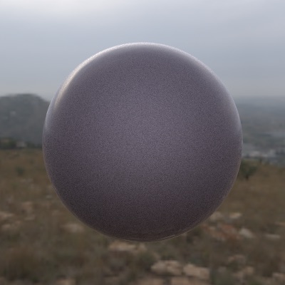
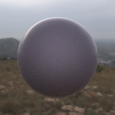
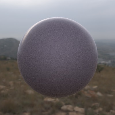
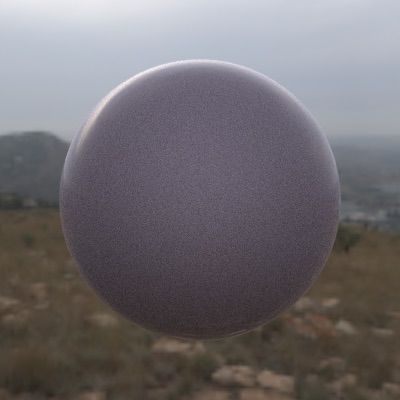
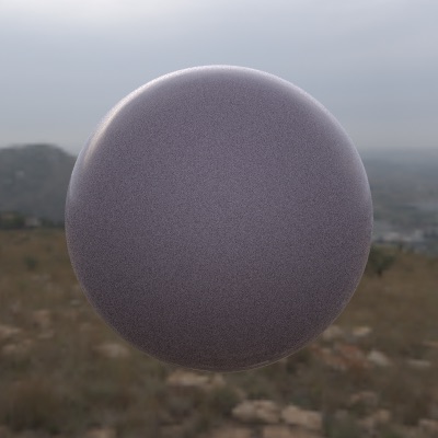
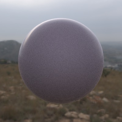
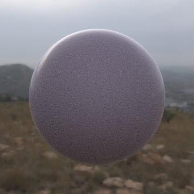
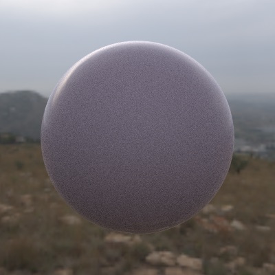
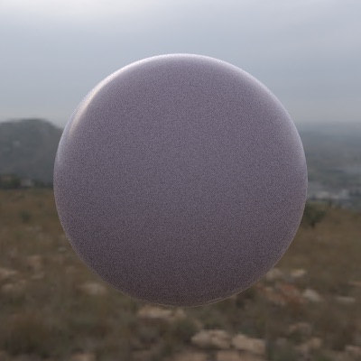
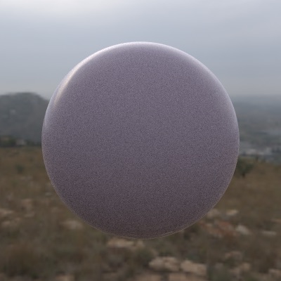
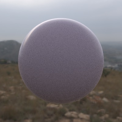
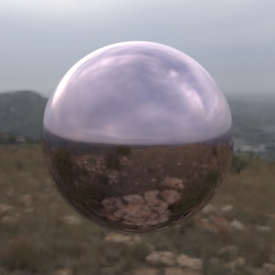
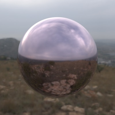
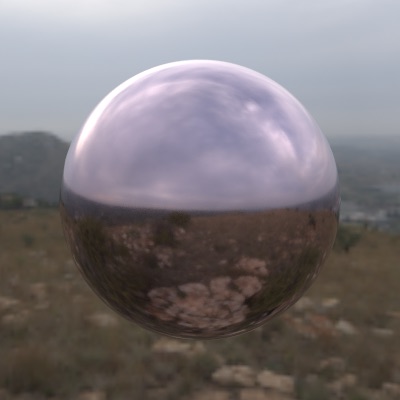
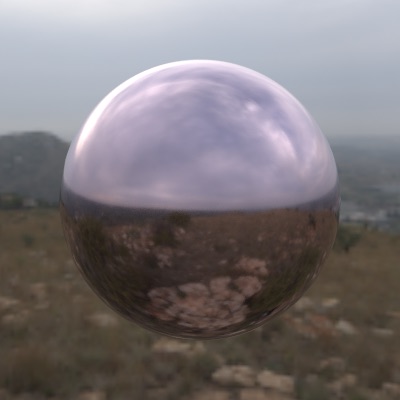
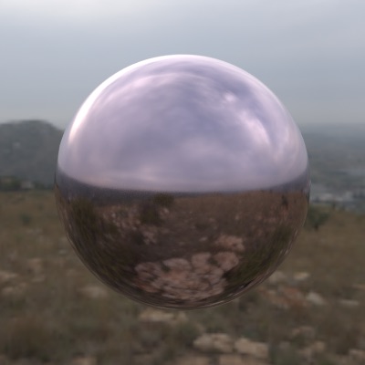
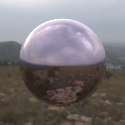
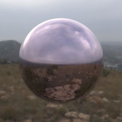
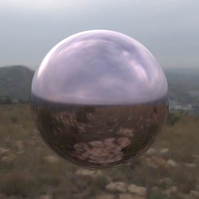
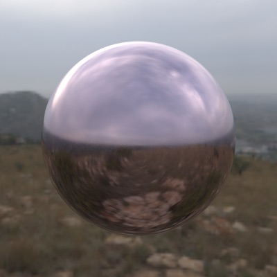
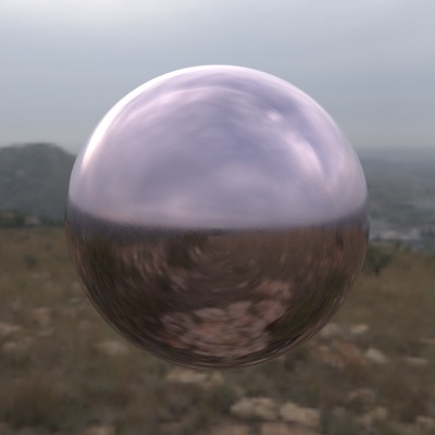
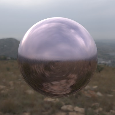
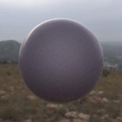
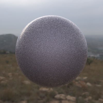
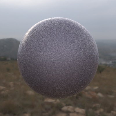
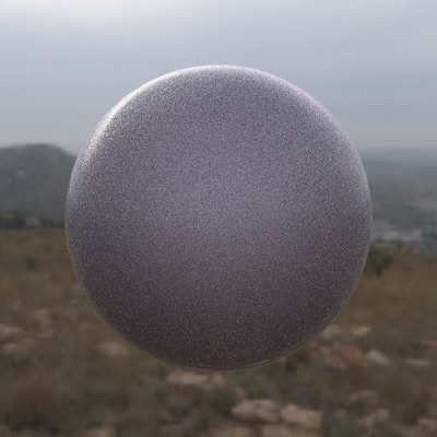
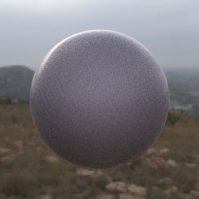
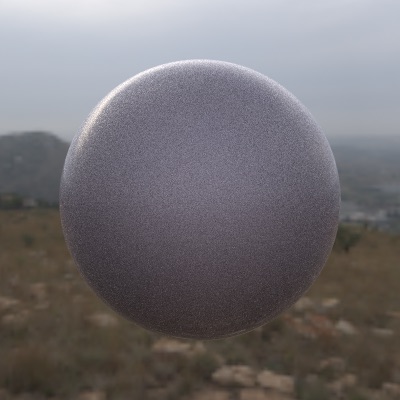
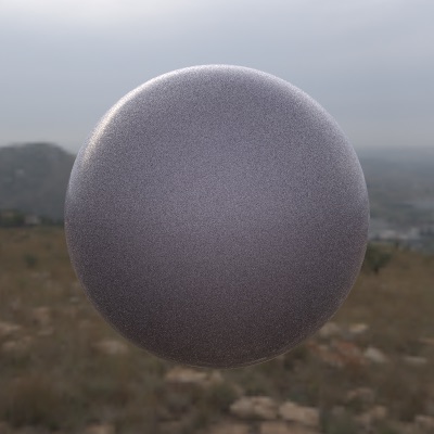
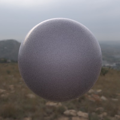
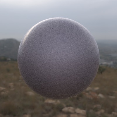
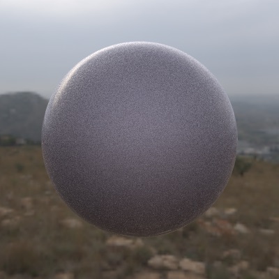
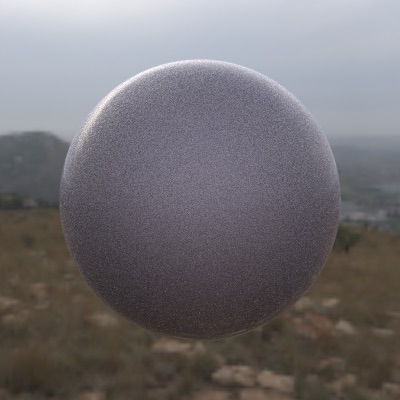
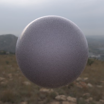
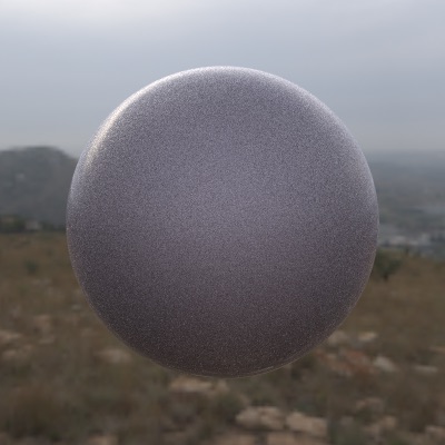
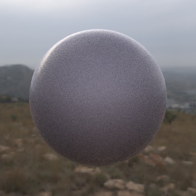
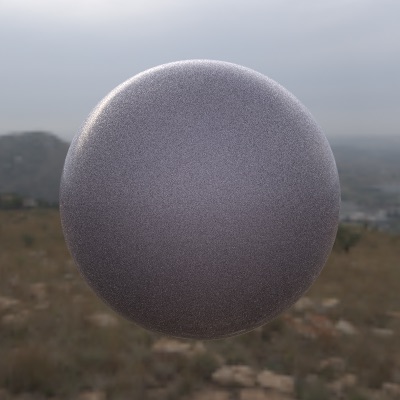
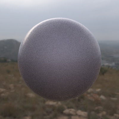
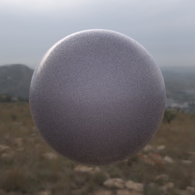
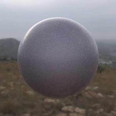
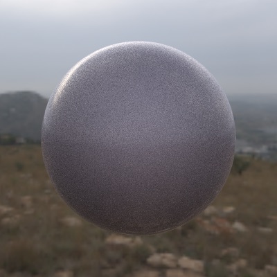
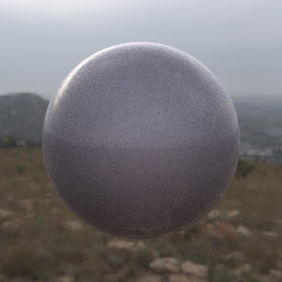
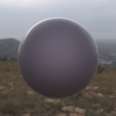
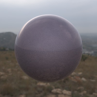
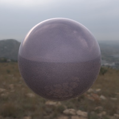
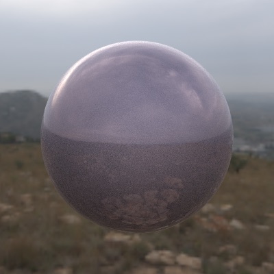
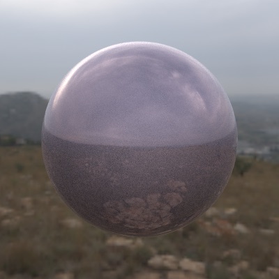
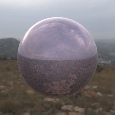
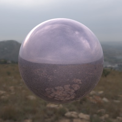
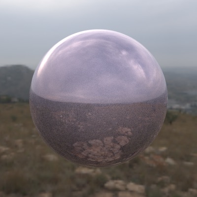
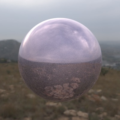
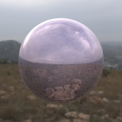
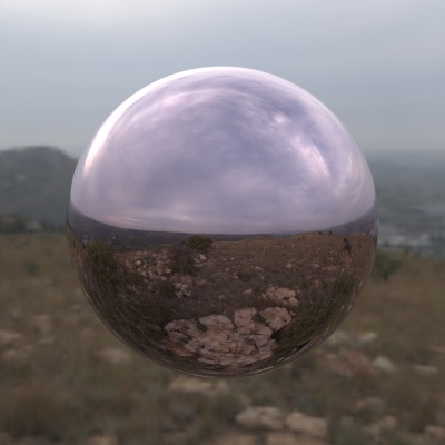
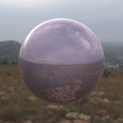
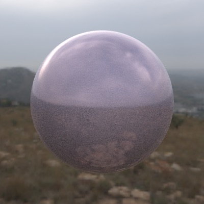
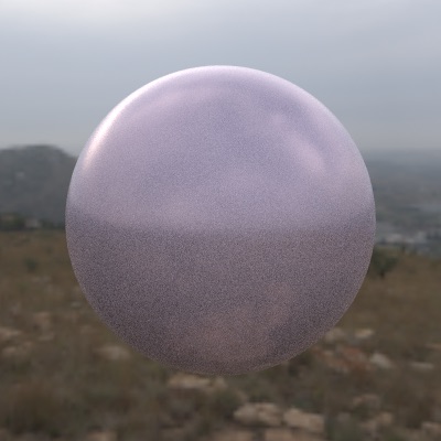
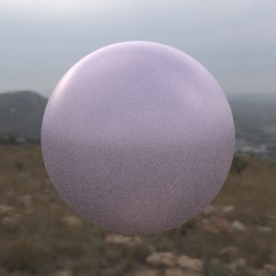
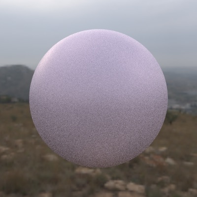
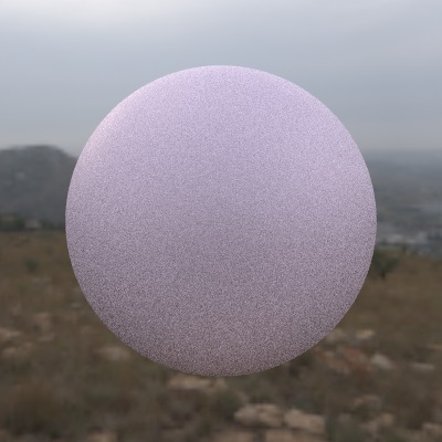
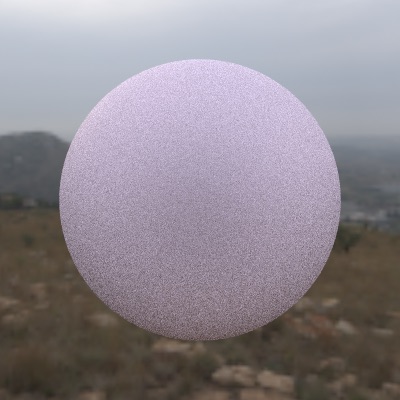
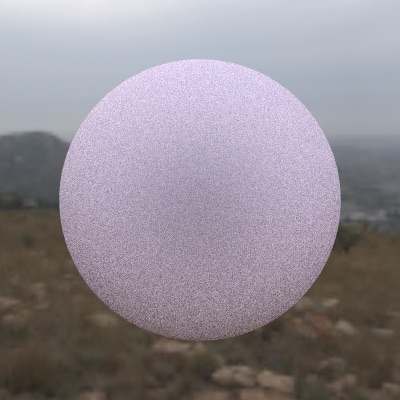
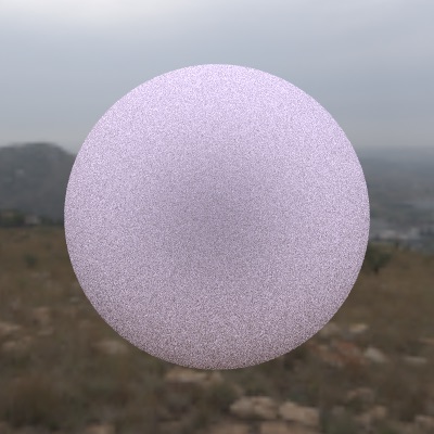
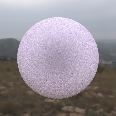
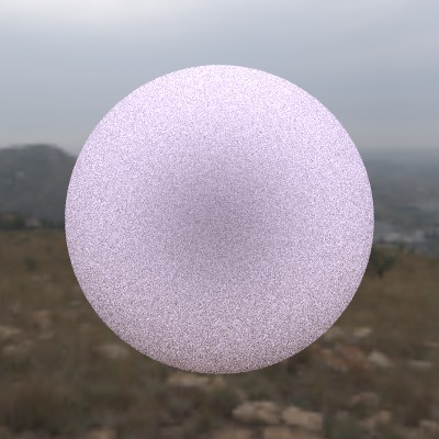
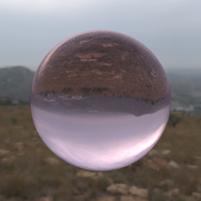
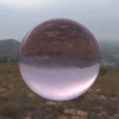
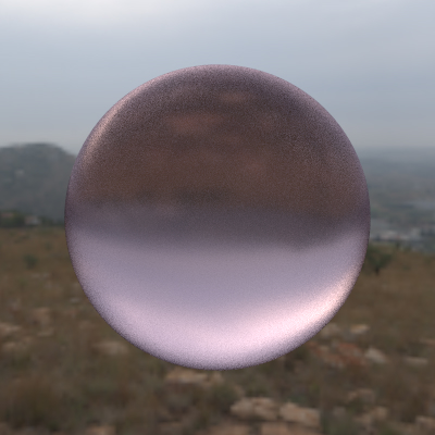
We want to model plastic material for our NES Console (which is made of plastic) that sometimes reflects light at grazing angles. The reflectance is modeled by coating a layer on the diffuse material. We faithfully follow the instruction from the UCSD homework to implement Disney Bsdf. This bsdf unifies all the material that we have implemented so far. Although not 100% physcially accurate, it still gives good and reasonable results.

Code:

src\bsdfs\disney.cpp

Subsurface

Subsurface 0.0	Subsurface 0.1	Subsurface 0.2
Subsurface 0.3	Subsurface 0.4	Subsurface 0.5
Subsurface 0.6	Subsurface 0.7	Subsurface 0.8
Subsurface 0.9	Subsurface 1.0	Subsurface 0.0

anisotropic

anisotropic 0.0	anisotropic 0.1	anisotropic 0.2
anisotropic 0.3	anisotropic 0.4	anisotropic 0.5
anisotropic 0.6	anisotropic 0.7	anisotropic 0.8
anisotropic 0.9	anisotropic 1.0	anisotropic 0.0

Cleatcoat

clearcoat 0.0	clearcoat 0.1	clearcoat 0.2
clearcoat 0.3	clearcoat 0.4	clearcoat 0.5
clearcoat 0.6	clearcoat 0.7	clearcoat 0.8
Subsurface 0.9	Subsurface 1.0	Subsurface 0.0

clearcoatGloss

clearcoatGloss 0.0	clearcoatGloss 0.1	clearcoatGloss 0.2
clearcoatGloss 0.3	clearcoatGloss 0.4	clearcoatGloss 0.5
clearcoatGloss 0.6	clearcoatGloss 0.7	clearcoatGloss 0.8
clearcoatGloss 0.9	clearcoatGloss 1.0	clearcoatGloss 0.0

Metallic

metallic 0.0	metallic 0.1	metallic 0.2
metallic 0.3	metallic 0.4	metallic 0.5
metallic 0.6	metallic 0.7	metallic 0.8
metallic 0.9	metallic 1.0	metallic 0.0

Roughness

roughness 0.0	roughness 0.1	roughness 0.2
roughness 0.3	roughness 0.4	roughness 0.5
roughness 0.6	roughness 0.7	roughness 0.8
roughness 0.9	roughness 1.0	roughness 0.0

Transmittance

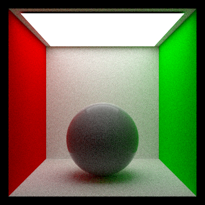
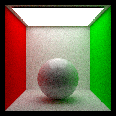
Comparison of Disney Coatting and Principle Specular for Plastic Material

Disney Coatting gives a little bit more realism than Principle Specular since the coatting layer of the Bsdf (not physcially accurate) reflects sufficient amount of light but not too much compared to Principle bsdf.

Other Features

CRT Effect

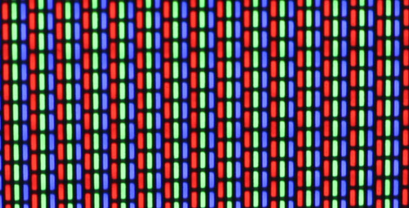
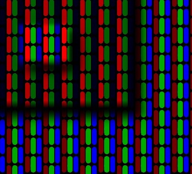
The old CRT TVs in 80s have an interesting effect, "CRT effect", which if we look closely to the screen, we can easily notice with our naked eyes that there are many separate red, green and blue pixels. And because the screen is curved, we can see some curved line strips in the screen. Although we can implement a texture class to simulate that effect, for the sake of simplicty, we modify the texture of screen byt multiplying it with a CRT pattern.