Computer Graphics - “Unknown Waters”

The Scene

The Final Render of the Scene

Scene name: Unknown Waters

Participants:

Lukas Auer
Johannes Schöneberger

Team name: Donphan

The scene shows a hybrid water and space ship heading through a portal to a seemingly familiar looking world through a giant portal while being surrounded by planets with weird auras and shapes. The style of the ship being a composition of the clashing styles of a science fiction esque space ship parts and a classic pirate ship further enhance the sense of journeying into the unknown.

Implemented Features

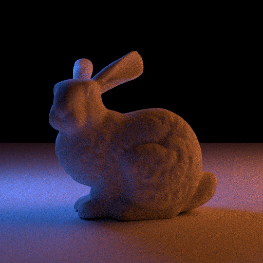
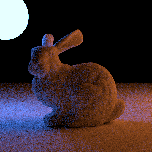
Area Lights

With Area Lights	With Emission Object

What is it?

Next event estimation is a very powerful tool to more reliably find light sources in a scene. Area Lights allow light sources other than point lights to be used for next event estimation. This can be used to create less noisy images and lead to more indirect light, especially if the light source is small.

Challenges

Area Lights require some changes in the next event estimation. This on its own is not very challenging since Lightwave already helps quite a lot to add area lights, such that we only needed to do two things.

Sample the surface of a shape
Adjust the intensity of the light according to the size of the shape

We achieved 1. by adding the function SampleArea to shapes, we wanted to use as Area Lights. Challenge 2. was a bit more tricky since we needed to figure out the surface area of the shapes, which changes with their scale. With a sphere, we solved this for example by using the cross product of the tangent and bitangent to scale the area.

Usage in the scene

We used area Lights to simulate some lights that originate outside of the scene. The fractal planet for example is illuminated from the top with an area light and the asteroids are also illuminated with area lights.

SDFs and Ray Marching

Fractal SDF rendered with space background

What is it?

SDFs can be used to represent objects using a function that returns the distance to the surface of the object at any given point in space. They are used for example in font rendering.
An SDF can be rendered by using Ray Marching, which uses the SDF of an object to march forward in space by the distance to the object until the distance is small enough to consider it a hit on the object.
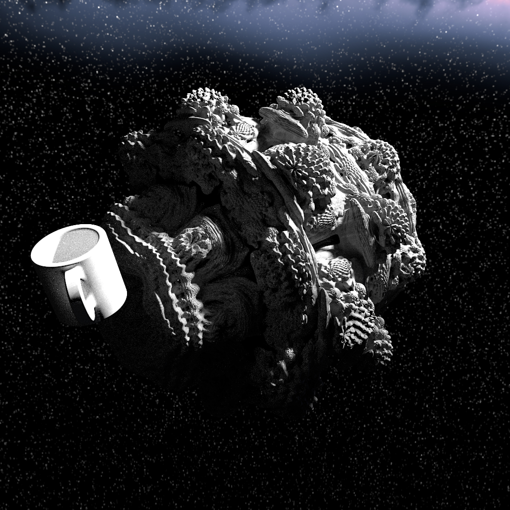
Since SDFs are just functions that compute the distance, they can be used to render complex mathematical shapes like fractals, as seen in the image above, and smooth combinations of primitive objects.

Challenges

The basic ray marching algorithm is rather simple to implement, but to get it to interact correctly with the existing ray tracing framework took some work.
Since hit positions are approximations when ray-marching SDFs, the hit points has to be moved away from the surface, in order to reduce the chance of self-intersections when casting multiple rays.

Another problem was how to represent SDFs in the scene. For this, we added a new object type to the XML scene configuration in the form of primitive SDFs like Spheres, Boxes and the Mandelbulb fractal in addition to operations that combine, inflate/round and transform SDF ojects contained as child nodes.

For computing the normal vectors of each hit point, one needs to compute the gradient of the distance estimator function of the SDF object. Our first implementation executed the distance estimator multiple times with a small offset in each coordinate direction to compute the gradient numerically. After that, we used a library that can be used to compute the gradient function directly to get accurate normal vectors.

UV mapping is also different with SDFs in comparison to using e.g. triangles in ray tracing, as one has to use different techniques to map the hit point on the SDF object to a UV coordinate. In our renderer we implemented only the Sphere mapping approach, that converts the hit point to sphere coordinates and only uses the two angles as coordinates.

Usage in the scene

SDFs are used in our scene to show an alien planet with a mandelbulb shape, which looks really intriguing with the texture we applied.

Volumetric Rendering

Volumetric fog

What is it?

Volumes are used to simulate particles that interact with light via absorption, scattering and emission. They can be used to model smoke, clouds and many other things.
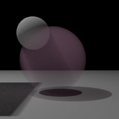
We only implemented homogeneous volumes, which can already be used for very nice effects. In the render above you can see a volumetric shadow that is created by the pink homogeneous fog.

Challenges

Implementing volumes posed many challenges to us.
First of all, we had to figure out how to add these volumes to the scene which proved itself to be a big challenge. In the end, we added a medium to the instance class which describes the medium that is inside the shape. At an intersection, we check if we enter or leave the shape and update the medium of the ray accordingly.
The next challenge was how to model the interactions with a medium. We decided that our integrator should always keep track of the medium in which a ray starts in. Then we intersect it with the scene. We also sample the medium for a distance at which we want to interact with it. If the intersection occurs after the sampled distance for a medium interaction, we interact with the medium by simulating scattering, absorption and emissions.

Usage in the scene

In our scene, the atmosphere of the planet in the foreground is created with a medium. The medium creates very nice light effects where the surface is bright which almost looks like a flair.
Also, the rings of the fractal planet are mediums, which have emissions this time.
Furthermore, the engine fire of the ship is created with a volume combined with a bsdf.

Portals

What is it?

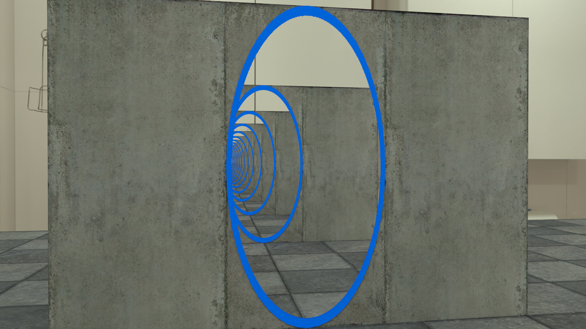
An "endless hole" effect using the portals feature

A popular method for travelling in science fiction is teleportation using portals, that links two places together like one is looking through a window to the other end. We though this would be a nice addition to our already science fiction and space travel inspired scene.
With portals, one can put some content in another part of the scene, but directly show it in the camera view using the mentioned window effect.
If a ray hits an instance marked as a portal and the UV of the hit lies on the portal shape mask, the ray will be re-emitted from the other, linked portal with the same relative position and location, thus making it look like the ray went right through. The portals also work in a nested fashion creating a sort of “endless hole” effect as can be seen in the example image above.

Challenges

The concept of a portal in ray-tracing is relatively simple, in that each ray just gets redirected, but the big challenge was integrating it into the existing ray-tracing framework and linking both portals in a way that the transformation of each portal can be known. We solved this by using a separate object for each pair of portals called a portal link that both portal instances register themselves to and which calculates the new rays.

Next Event estimation is not included in the current implementation of the feature, as it requires more work to work properly.

Usage in the scene

This feature was used in the scene to take a look at a different world that a space ship will journey to.

Shading Normals

Without Shading Normals	With Shading Normals

What is it?

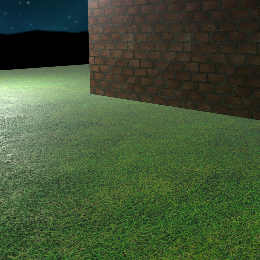
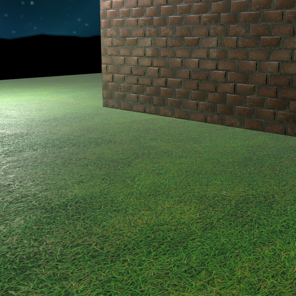
Modelling an object while keeping all the extremely fine details, like scratches, bumps, etc. consumes extremely many polygons, so many models come with a normal map. This maps how the normal vectors on the surface should look to approximate the finer details on the surface.
In our opinion, this is a must have feature, as it enhances the look of model surfaces a lot.
The implementation uses the values stored in the texture as local normal vectors pointing away from the surface and transforms them from shading space to world space instead of the real surface normal.

Challenges

As we are working with blender for creating scenes more easily, this implmentation should ideally be relatively close to how blender does it. This, however, is not that easy, as blender does many more complex things, so some trial and error had to be done to get relatively close. The first approaches tried extracting rotation from the normal vector from the map and applying that to the existing normal vector in world space, but in the end, the simplest approach was to apply the matrix transpose to the desired normal vector and recompute the tangent and bitangent vector afterwards.

Usage in the scene

Nearly every material used on the models in the scene use some normal map to improve the look of their surfaces.

Thinlens Camera

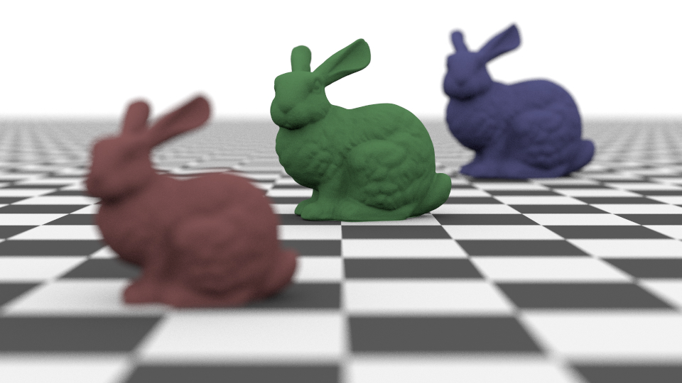
Perspective camera	Thinlense camera with high apature radius

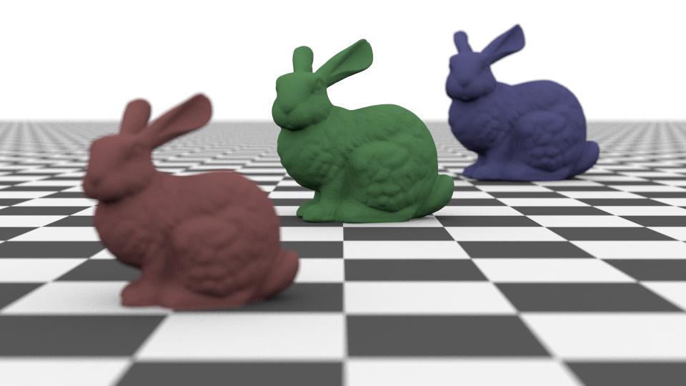
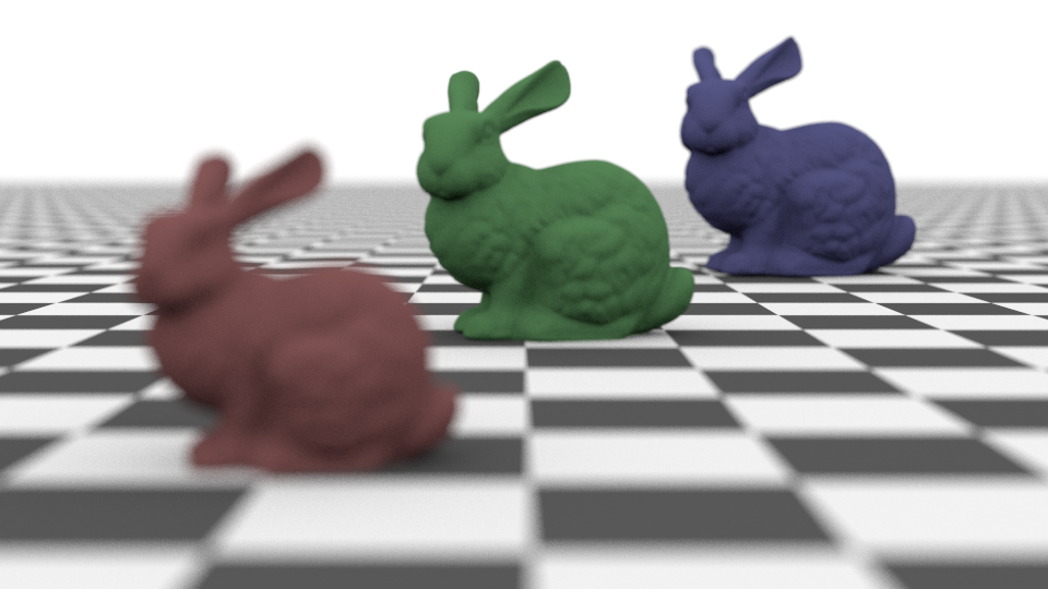
Thinlense camera with smaller apature radius	Thinlense camera with higher focal distance

What is it?

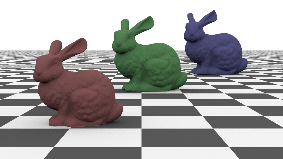
The thinlense camera is an alternative camera that more realistically models actual cameras. The perspective camera assumes the focal point to be infinitely small while a thinlense camera has a “focal circle”. This leads to having only objects at a certain depth be sharp, and the further away objects are from this “focal plane”, the more blurry they become.
The thinlense camera model has two parameters:

The adpature radius, desribes how large the scatter area for the ray origin is
The focal distance, descibes at what distance the image is sharp

Their influence can also be seen in the renders above.

Challenges

Figuring out how the math behind the thinlens camera model works to create the right samples was not that easy. The Pbrt book helped us a lot here.

Usage in the scene

We actually did not use the thinlense in our render because it looked strange to have our objects not sharp as this would take away from the fractal, for example.

Image Denoising

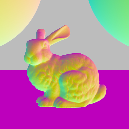
Albedo	Normals

Noise Output	Denoised Output

What is it?

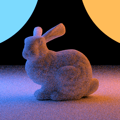
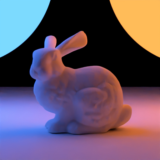
Open Image Denoise is an open-source library by Intel to denoise the output of a ray tracer. It requires an albedo image, a normal image and the output of the ray tracer to create high-quality denoising results. You can see the result of the Open Image Denoise library in the example above.

Challenges

As with any library, it needs a bit of reading to understand the provided functions and how to use them. After a bit of testing, the implementation of this feature was very straightforward.

Usage in the scene

In our render the denoising is used to significantly reduce the required number of samples per pixel. This speeds up our renderer and creates a smooth final image.

Used Resources

Further Comments

Can the university provide computers next time? xD

Hi Mum <3

Here is a bonus render of our team spirit pokemon: