Project Overview
Scene: The Last Stand
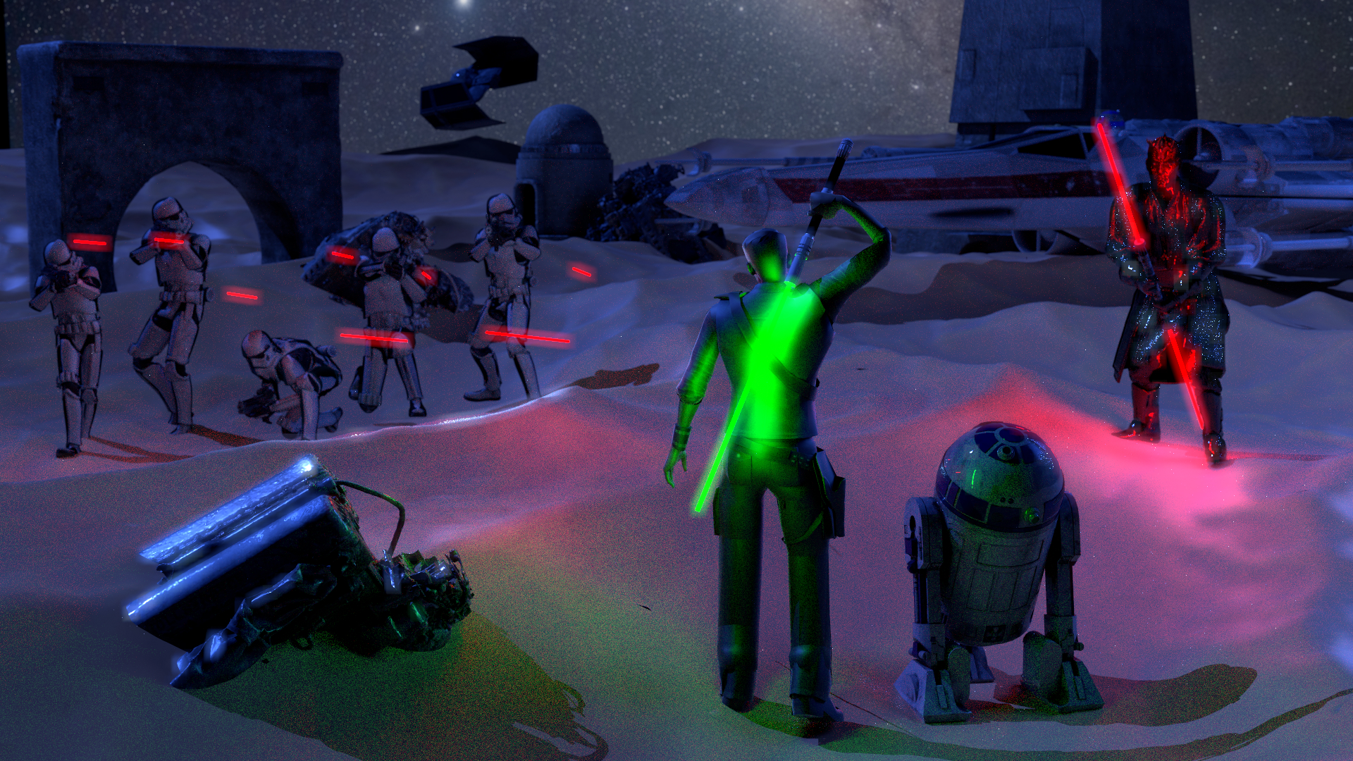
This project is inspired by our shared passion for the Star Wars universe. Arham's experience comes from playing the Star Wars games, while Moid Huda's connection is rooted in repeatedly watching the complete film series. This contrast in engagement motivated the crossover at the center of the scene: the Jedi Cal Kestis from the games confronting the Sith Lord Darth Maul from the movies.
The scene is set in a vast, desolate desert to convey isolation, helplessness, and the unforgiving nature of fate. Wreckage and debris scattered across the landscape suggest prior destruction and ongoing conflict. Although an X-wing starship stands nearby as a possible escape, the Jedi must first cross a hostile force of Imperial stormtroopers, with the distant arrival of another Imperial ship further worsening the odds.
Accompanied by his loyal companion R2-D2, the Jedi prepares for an inevitable confrontation. Rather than depicting action, the scene captures a moment of resolve—the calm before a battle that is almost certainly lost. A detail that may go unnoticed is the positioning of light and color: the opposing glow of red and green not only separates enemy from hero, but visually reinforces the moral and emotional divide that defines the Jedi's final stand.
Rendering Statistics
Hardware: MacBook Air M3
Total Render Time: 5089.57 seconds (~1 hour 25 minutes)
Performance Breakdown:
- Ray-Scene Intersection: 55.1% (9.7 billion intersection tests)
- Triangle mesh intersections: 33.8% (63 billion tests)
- Rectangle intersections: 0.7% (9.7 billion tests)
- Volume Transmittance: 25.1% (2.9 billion evaluations)
- BSDF Sampling: 9.4% (6.5 billion samples)
- Principled BSDF: 8.6% (5.9 billion samples)
- Light Sampling: 1.8% (6.5 billion picks)
- BSDF Evaluation: 1.1% (1.4 billion evaluations)
Process and Development
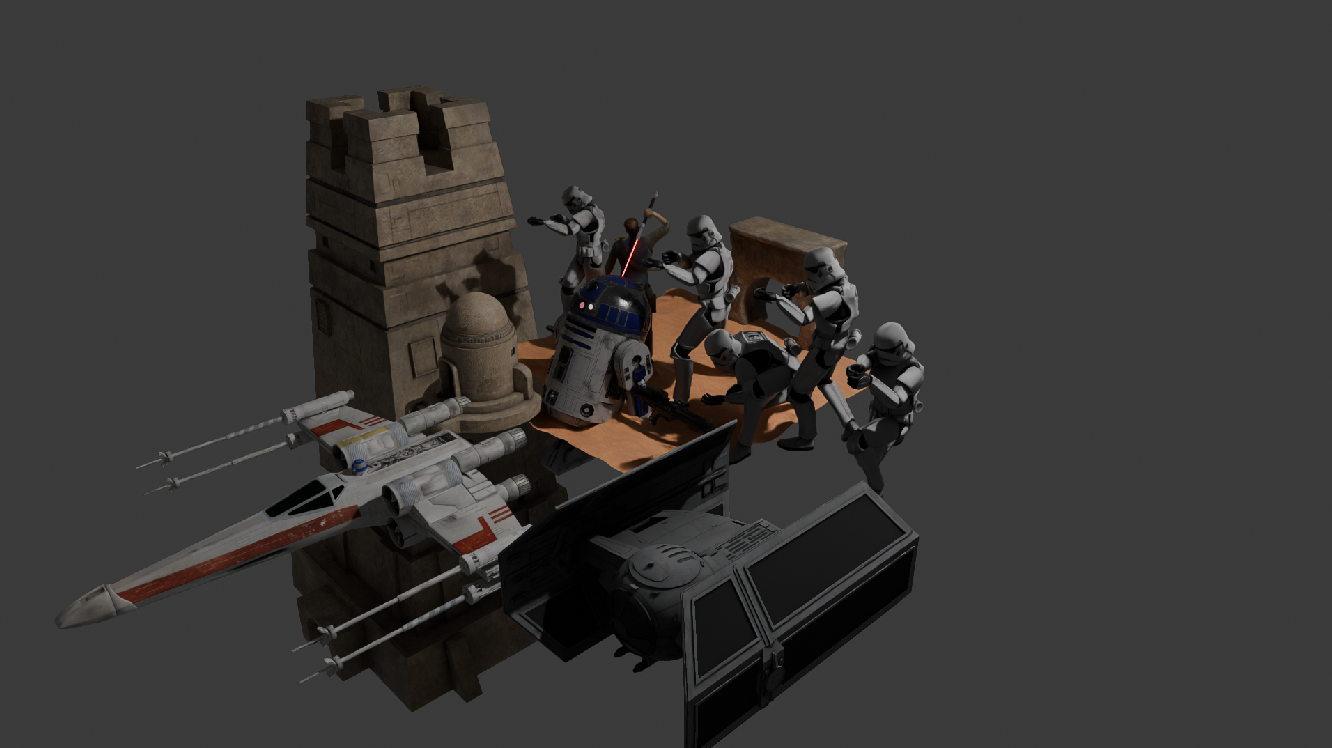
Our process began by simply bringing all the models we had collected into a single Blender scene. In the first image shown below, we placed everything close together without worrying about composition or storytelling. The goal at this stage was to make sure that all assets could be imported and rendered correctly. This helped us catch early issues related to scale, materials, and compatibility before moving on to building the actual scene.
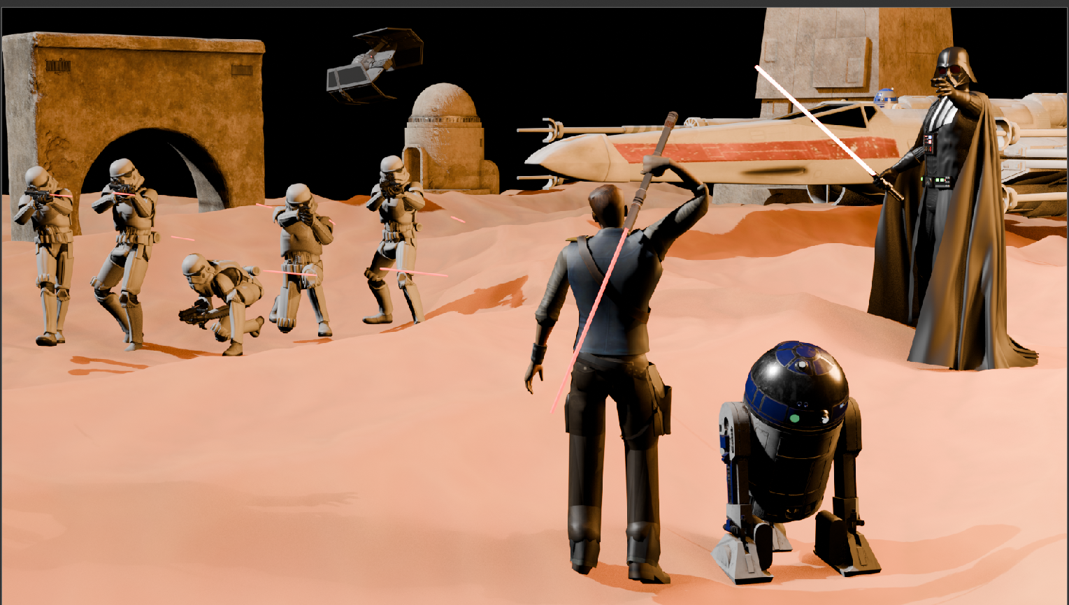
In the second image, we show an early version of the full scene that we initially imagined very differently. At first, the environment was set during the day, and the villain was Darth Vader. However, the Darth Vader model we obtained was not compatible with our export workflow and file parser, which made it unusable. More importantly, we realized that a bright daytime setting did not support the tragic and hopeless mood we wanted to convey. The strong sunlight also reduced the visual impact of the lightsabers, which are meant to be a key emotional and visual element. This led us to rethink both the lighting and the choice of antagonist.
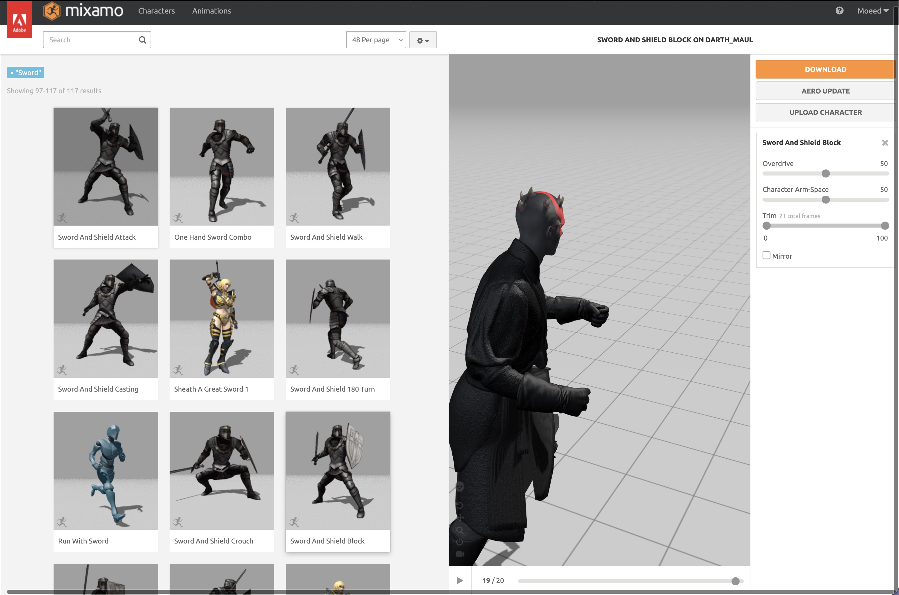
The third image focuses on character posing. After deciding on Darth Maul, we used Mixamo to experiment with several poses and animations. Since Darth Maul wields a dual-bladed lightsaber, we chose a pose that felt aggressive, balanced, and visually dominant. The selected pose was then exported and applied to the model in Blender, helping the character feel grounded and ready for confrontation within the scene.
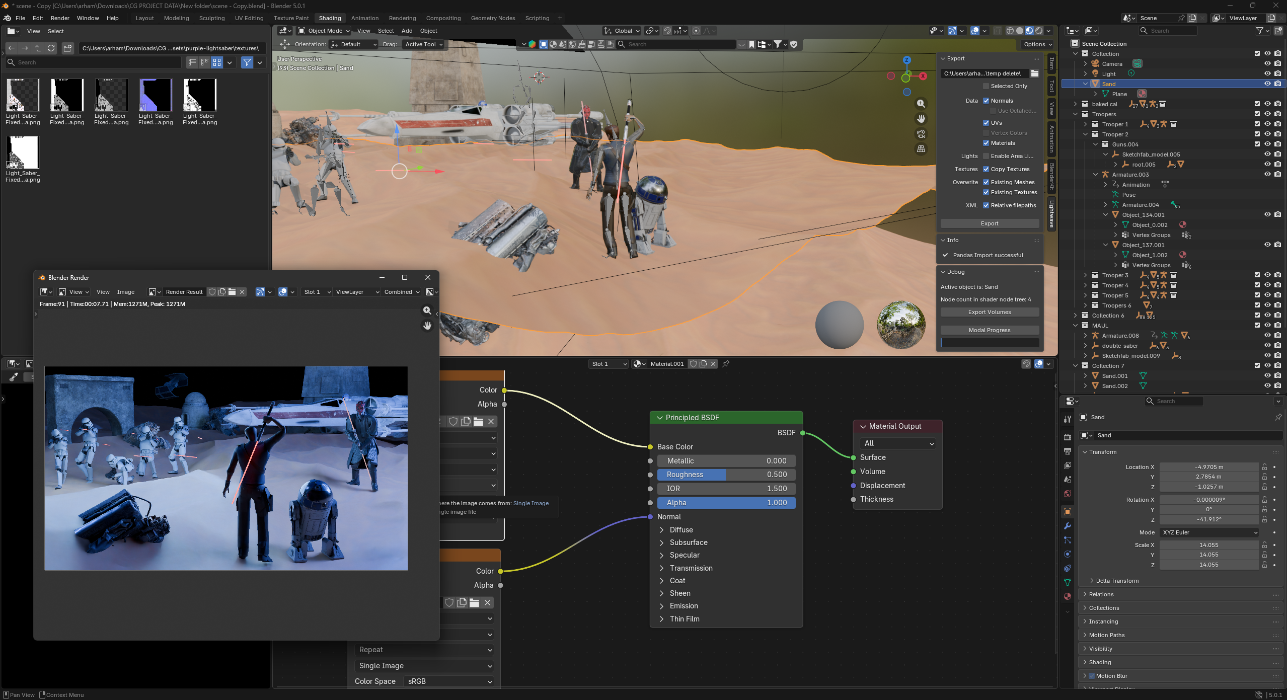
The final image shows the completed setup inside Blender. At this stage, we focused on refining the placement of elements, adjusting the lighting, and setting up the camera to capture the moment just before the battle begins. This final step brought together all previous decisions, resulting in a scene that reflects both our technical exploration and the emotional narrative we set out to create.
This project showcases the implementation of advanced rendering features in the Lightwave ray tracing engine. The renderer supports physically-based materials, realistic camera models, advanced sampling techniques, and post-processing effects.
Implemented Features
Navigate through the menu above to explore each feature in detail, including implementation notes, rendered examples, and technical challenges.
Camera Features
Advanced camera models for realistic optical effects.
Realistic Camera (Physical Lens)
Realistic Camera
Perspective Camera
Description
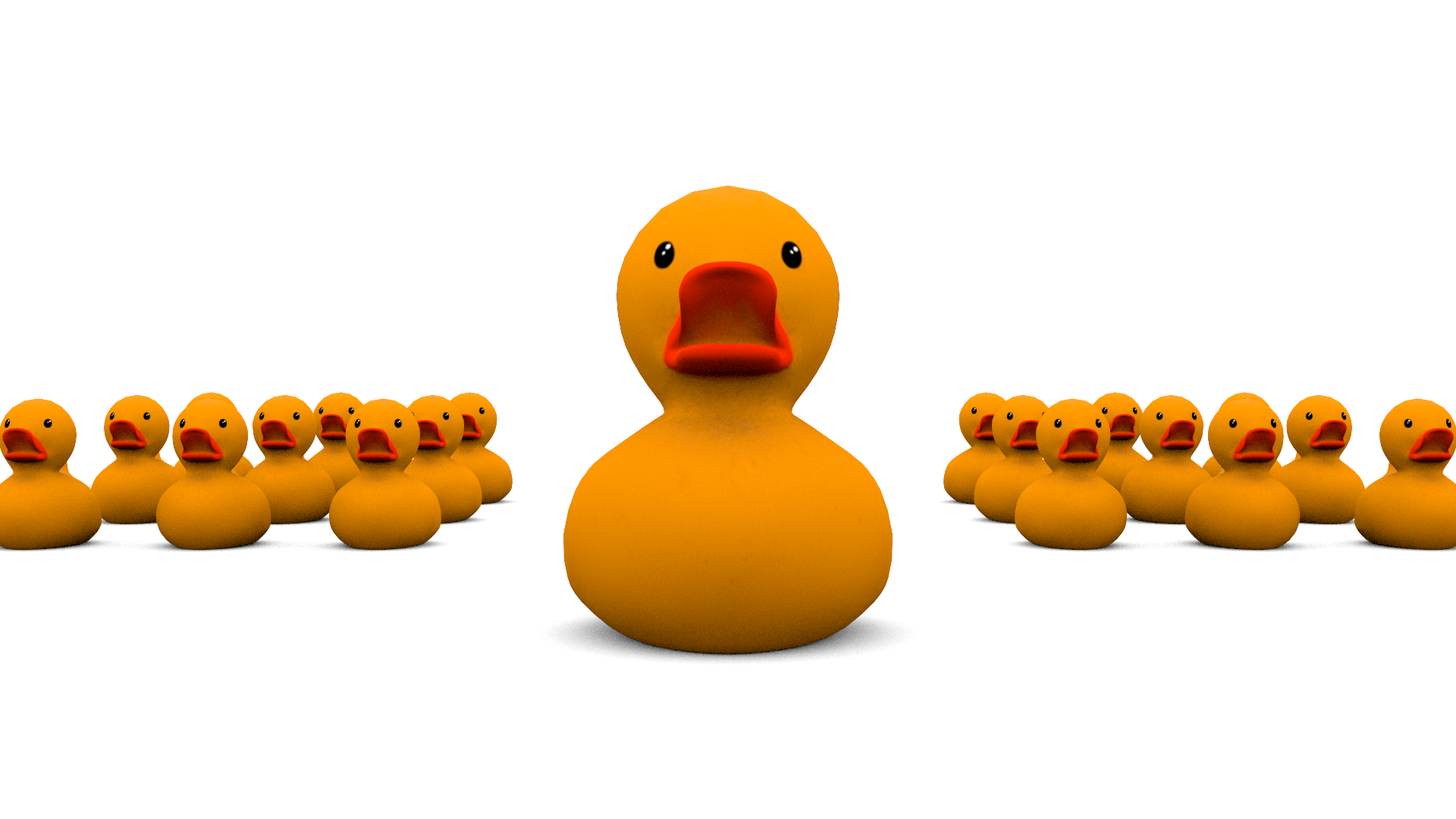
Implements a physically accurate camera model based on real lens systems. The camera simulates multi-element lens optics, including realistic depth-of-field, focus distance, aperture diameter, and optical aberrations. Lens data is loaded from industry-standard .dat files containing specifications for real camera lenses.
Implementation Summary
Modified Components:
src/cameras/RealisticCamera.cpp - Complete camera implementation- Lens system parser for .dat files
- Ray tracing through multi-element lens system
- Exit pupil bounds computation for importance sampling
- Weight calculation with proper throughput scaling
Key Features:
- Traces rays through each lens element (front-to-back and back-to-front)
- Handles refraction at each air-glass interface using Snell's law
- Computes exit pupil bounds for efficient sampling
- Applies cos⁴θ vignetting and aperture-based light falloff
- Supports adjustable aperture diameter and focus distance
Biggest Challenge
Weight Normalization and Brightness Matching: The most challenging aspect was getting the exposure correct. Initially, images were 15-40x too dark because the weight calculation only accounted for relative vignetting but not the absolute light-gathering power of the lens. The issue was traced to the exit pupil area being measured in tiny physical units (square micrometers) without proper normalization.
The solution involved:
- Computing a normalized weight based on film area and lens-to-film distance
- Adding an empirically-tuned exposure scale factor (15.0x) to match perspective camera brightness
- Converting from physical lens area units to solid angle units comparable to pinhole cameras
- Extensive debugging with weight value logging to identify the 50-100x scaling issue
Projective Camera (Thin Lens)
Description
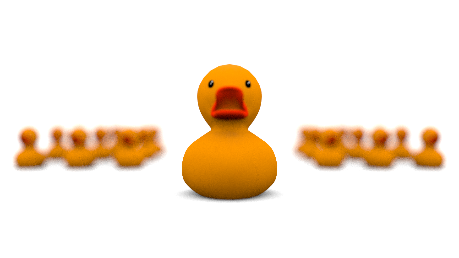
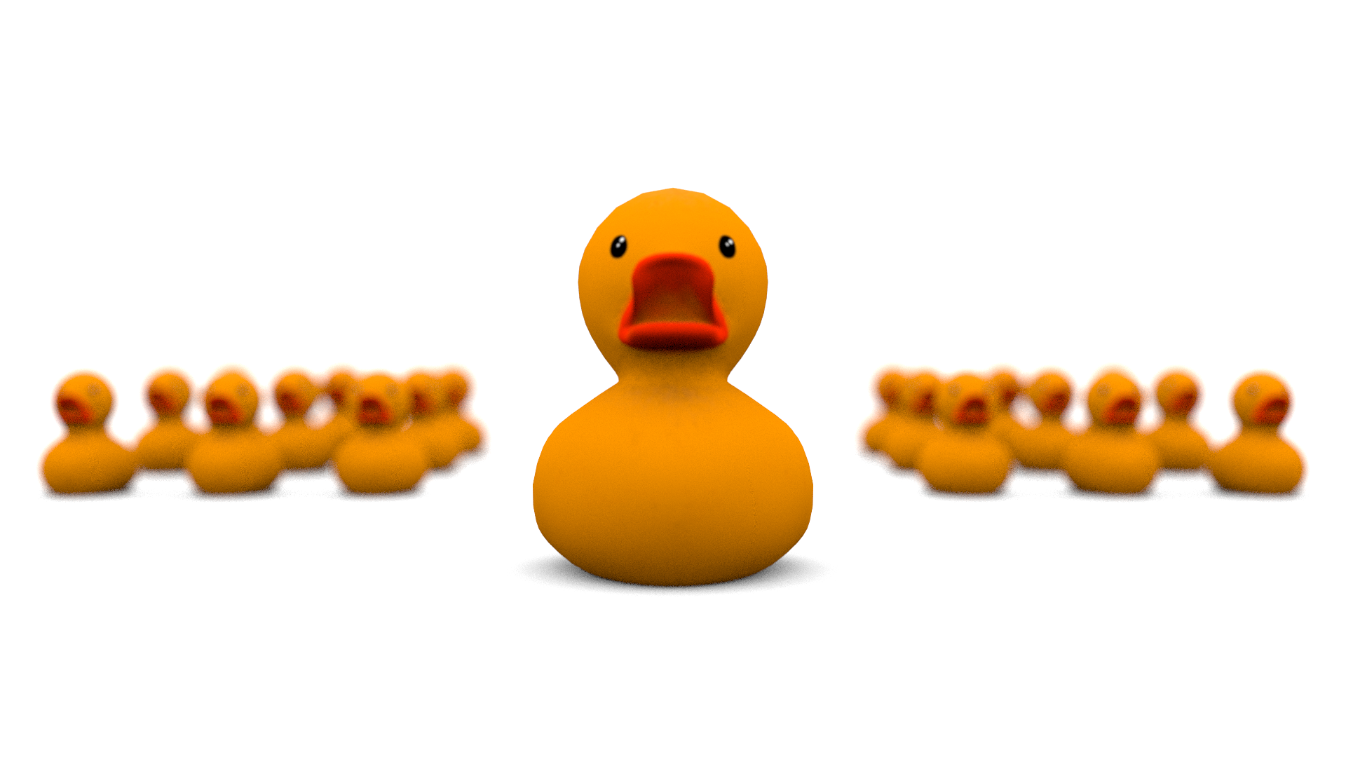
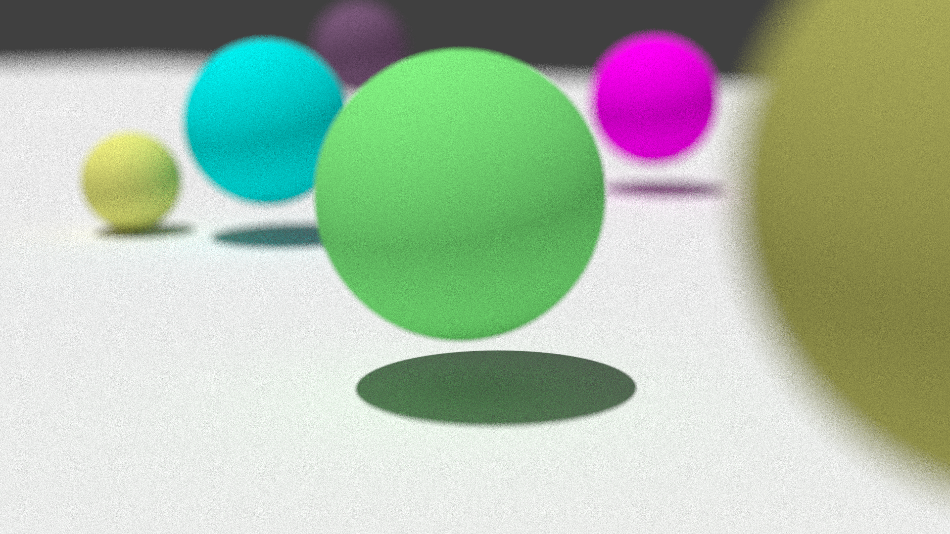
Implements depth-of-field effects using the thin lens approximation. Unlike the realistic camera which simulates actual lens elements, this camera uses a simplified optical model with a single focal plane and adjustable lens radius. Objects at the focus distance appear sharp, while foreground and background elements are progressively blurred.
Implementation Summary
Modified Components:
src/cameras/ProjectiveCamera.cpp - Thin lens implementation- Lens sampling for ray distribution
- Focal plane intersection computation
- Adjustable lens radius and focal distance parameters
Algorithm:
- Generate primary ray through film point to focal plane
- Sample point on circular lens aperture
- Compute ray from lens sample through focal point
- Rays converge at focal distance, creating sharp focus
- Larger lens radius = stronger depth-of-field effect
Biggest Challenge
Focal Distance Calibration: The main difficulty was determining the correct focal distance for a given scene. Unlike real cameras with autofocus, the focal distance must be manually calculated or estimated. For complex scenes, this required iterative testing with different focus values and understanding the relationship between scene depth, lens radius, and blur amount. The challenge was compounded by the need to balance artistic control with physical accuracy.
Small Aperture (Deep DoF)
Large Aperture (Shallow DoF)
Perspective No DoF
Large DoF
Rendering Features
Advanced sampling and lighting techniques for high-quality renders.
Sobol Low-Discrepancy Sampling
Independent Sampling (16 spp)
Sobol Sampling (16 spp)
Description
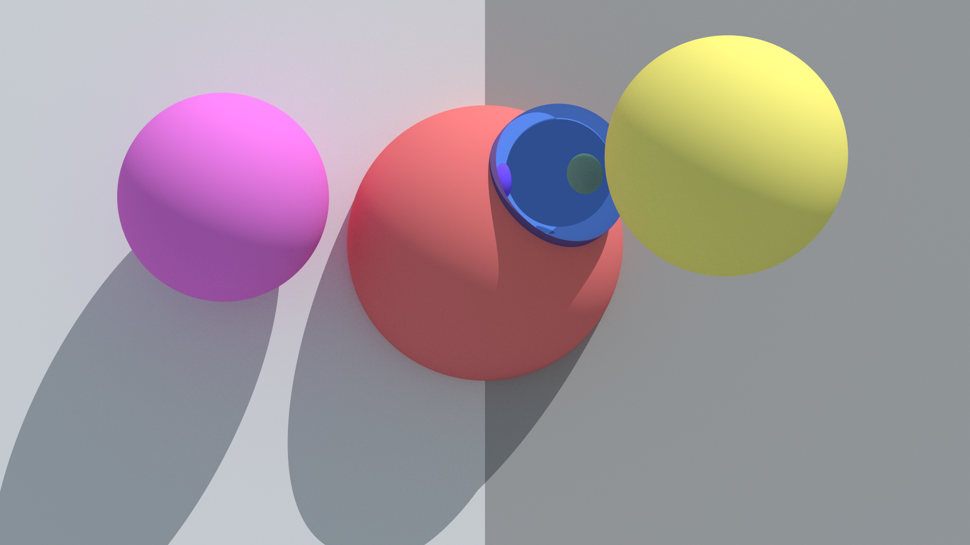
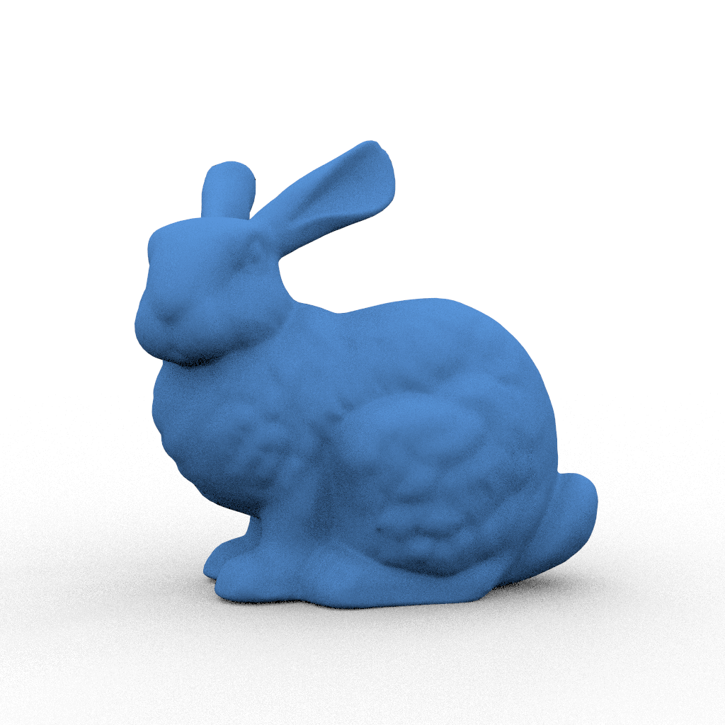
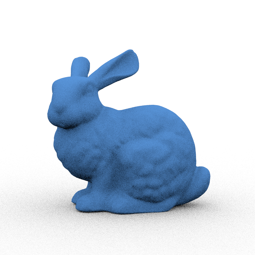
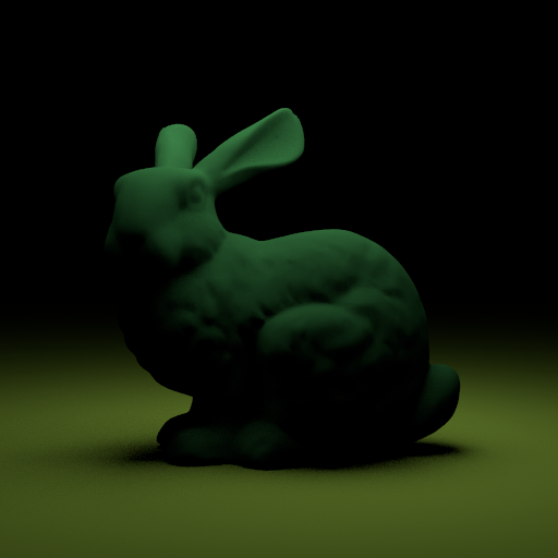
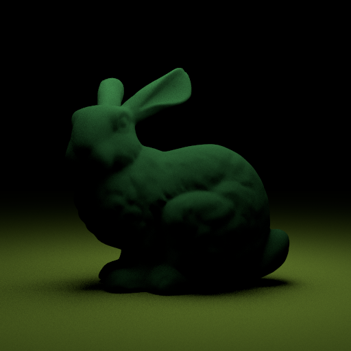
Implements Sobol quasi-random sequences as an alternative to independent (pseudo-random) sampling. Sobol sequences are low-discrepancy sequences that distribute samples more evenly across the sampling domain, significantly reducing noise for the same number of samples per pixel. Both images above use exactly 16 samples per pixel, demonstrating that Sobol sampling produces much cleaner results at equal computational cost. This improvement is especially noticeable in indirect lighting and shadow regions.
Implementation Summary
Modified Components:
src/samplers/sobol.cpp - Complete Sobol implementationsrc/samplers/sobolmatrices.cpp - Pre-computed generator matrices- 1024-dimensional Sobol sequence with 52-bit resolution
- Support for multiple scrambling methods (Binary Permute, FastOwen, Owen)
Key Features:
- Direction numbers from Joe and Kuo (up to 1024 dimensions)
- Efficient bit operations for sequence generation
- Per-pixel and per-sample seeding for decorrelation
- Optional Owen and FastOwen scrambling for improved distribution
- Maintains low discrepancy while allowing random permutations
Biggest Challenge
Scrambling and Correlation Artifacts: The most challenging aspect was implementing proper scrambling to avoid correlation artifacts between adjacent pixels. Initial implementations showed visible structured patterns in the noise, especially in gradients and shadow penumbras. The issue stemmed from using the same Sobol sequence for neighboring pixels.
The solution required:
- Implementing Owen scrambling with nested random digit permutations
- Using hash-based seeding combining pixel coordinates and sample index
- Understanding the trade-off between scrambling strength and sequence quality
- Testing multiple scrambling strategies (None, Binary Permute, FastOwen, Owen)
- Balancing the benefits of low-discrepancy with the need for pixel independence
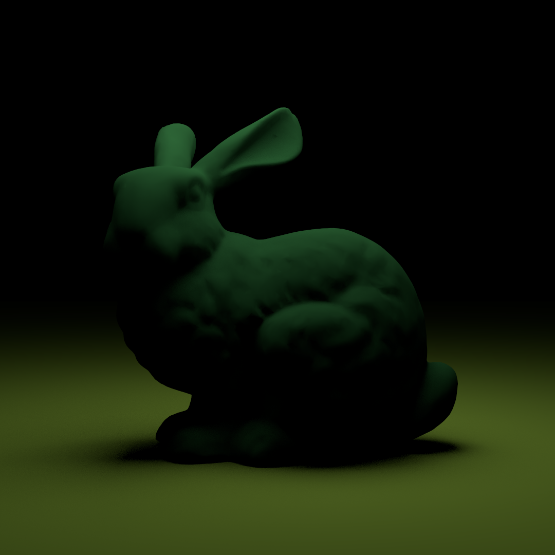
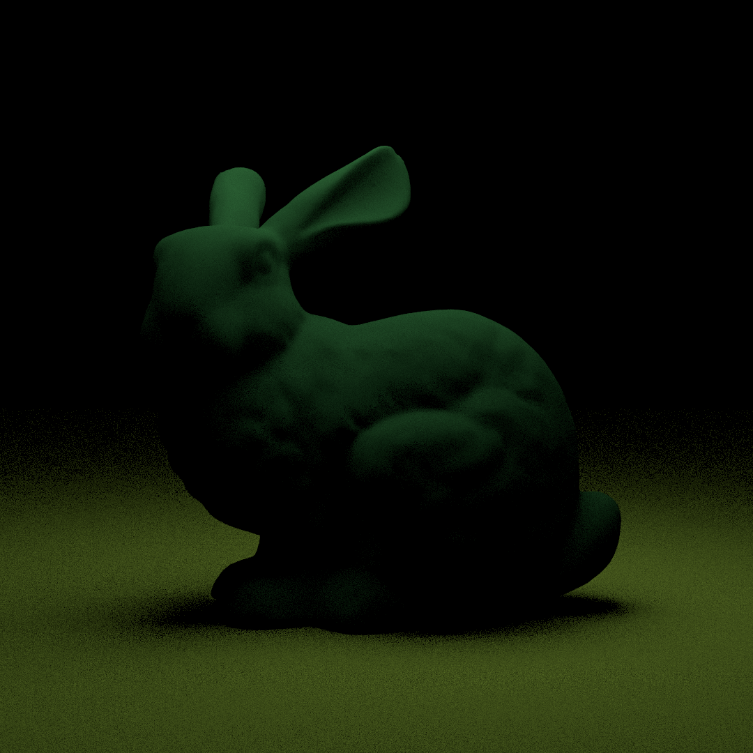
Noise comparison at 64 SPP and 256 SPP: Sobol sampling converges significantly faster
Area Light Sampling
Description
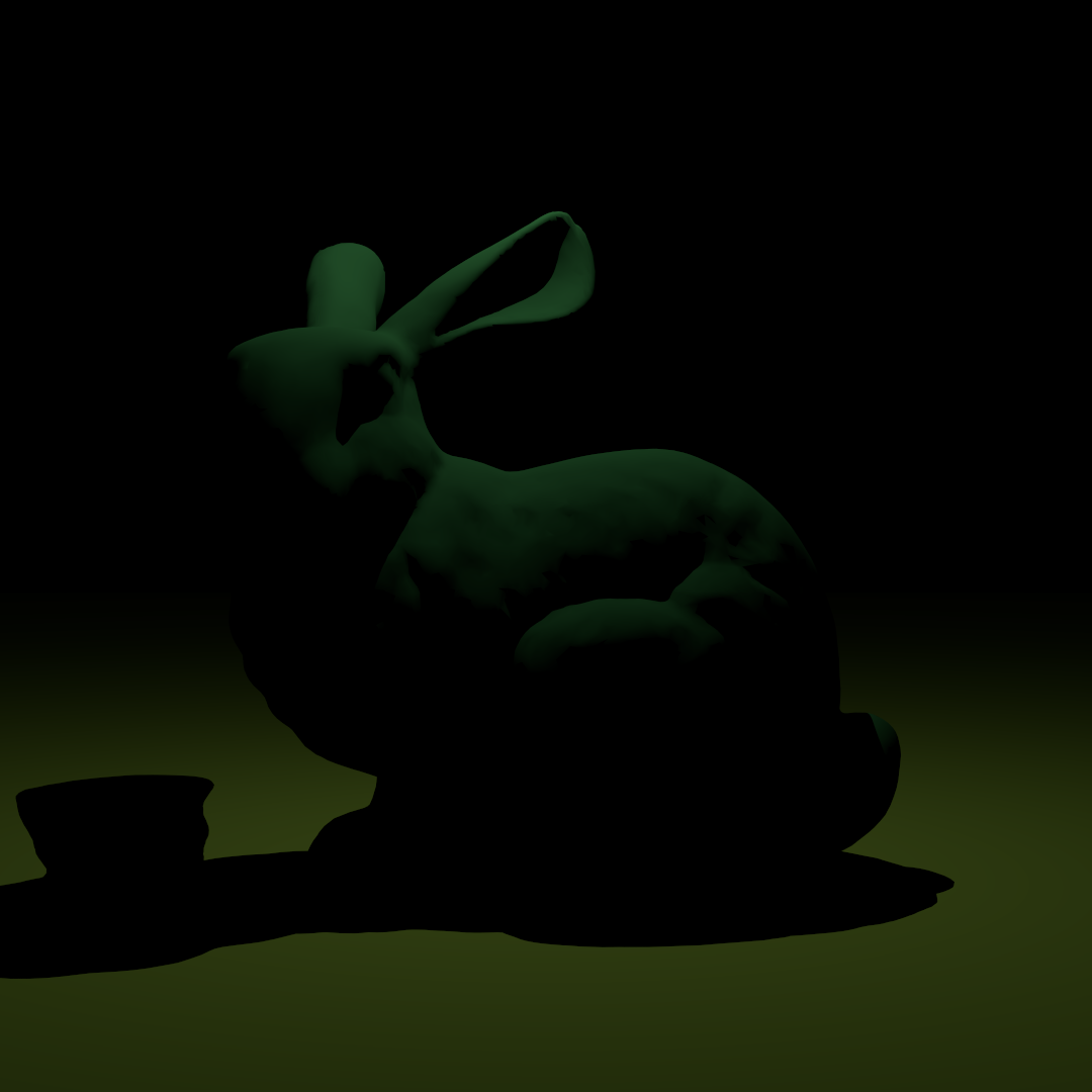
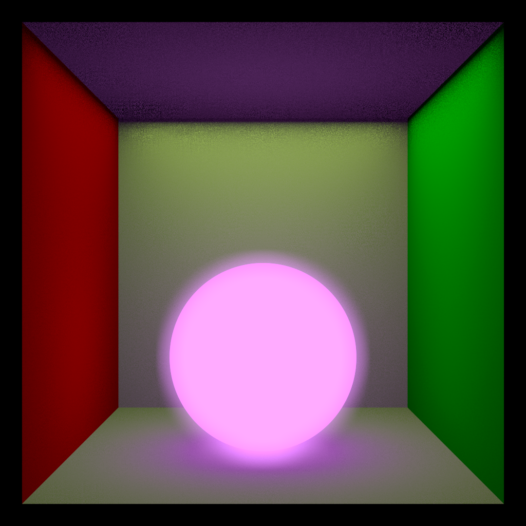
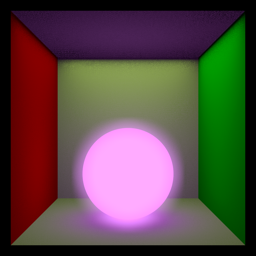
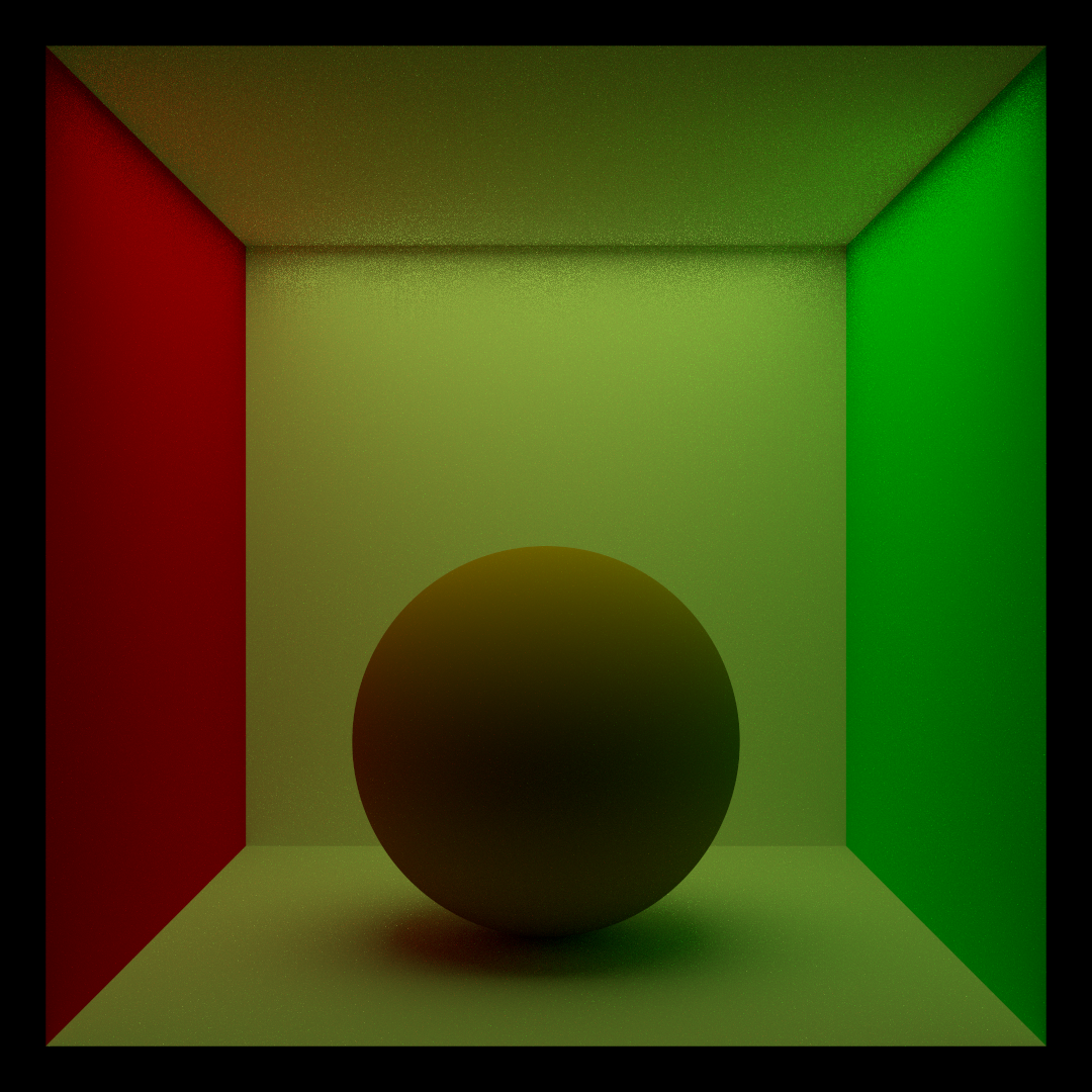
Implements area light sources that emit light from a geometric surface (spheres, rectangles, meshes) rather than from a single point. This creates realistic soft shadows with smooth penumbra regions. The implementation includes importance sampling of the light surface and proper geometric term evaluation for accurate energy distribution.
Implementation Summary
Modified Components:
src/lights/area.cpp - Area light implementationsrc/shapes/sphere.cpp - Sphere area sampling methodsrc/shapes/rectangle.cpp - Rectangle area sampling- Integration with path tracer's next-event estimation
- Visibility testing for shadow rays
Key Features:
- Uniform area sampling with proper PDF computation
- Cosine-weighted importance sampling for Lambertian emitters
- Geometric term (cosθ / r²) for light falloff
- Multiple importance sampling for variance reduction
- Support for textured emission (image-based lighting)
Biggest Challenge
Sphere Area Sampling Consistency: The biggest challenge was implementing correct and efficient sphere area sampling. The initial implementation used simple spherical coordinate sampling, which created visible artifacts at the poles (non-uniform distribution). Additionally, computing the correct PDF for oriented area sampling (where the light's facing direction matters) required careful geometric analysis.
The solution involved:
- Using rejection sampling on the hemisphere visible from the shading point
- Properly handling the solid angle PDF conversion to area PDF
- Implementing efficient sphere-point distance and normal computation
- Testing with Cornell box scenes to verify shadow softness
Point Light (Hard Shadows)
Area Light (Soft Shadows)
Emission Texture (Noisy)
Area Light (Less Noise)
Bloom Post-Processing
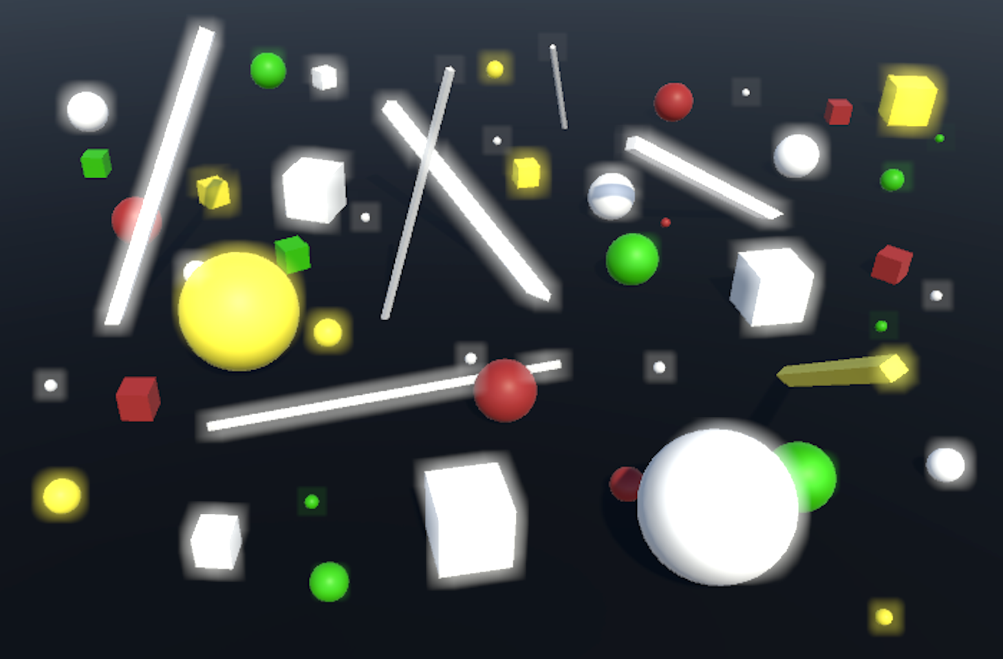
With Bloom Effect
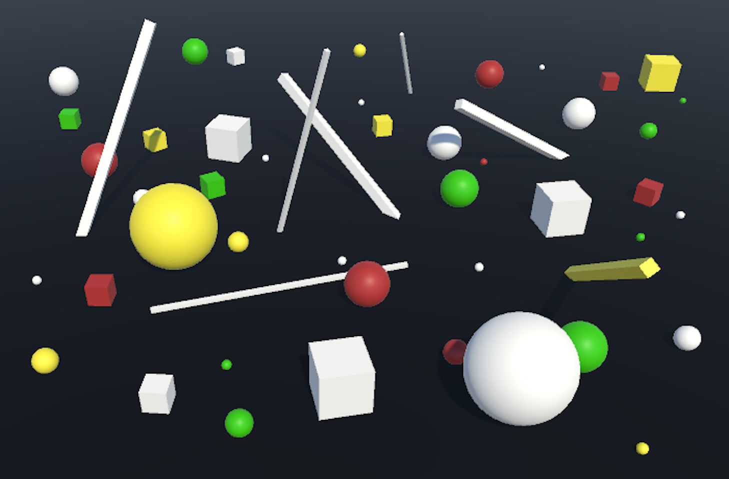
Without Bloom
Description
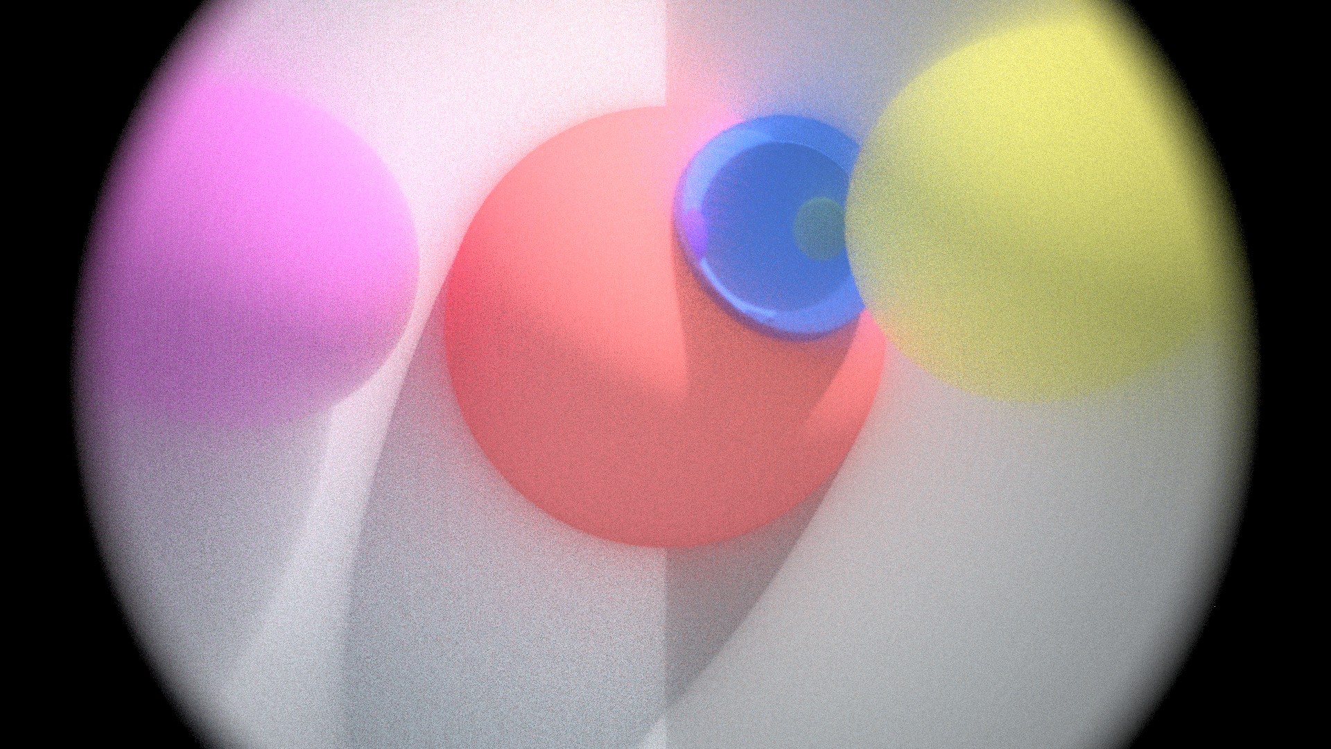
Implements a bloom post-processing effect that creates realistic glow around bright light sources and reflections. This simulates the scattering of light in real camera lenses and the human eye. The effect extracts bright regions above a luminance threshold, applies Gaussian blur, and composites the result back onto the original image.
Implementation Summary
Modified Components:
src/postprocesses/bloom.cpp - Complete bloom implementation- Configurable luminance threshold for bright extraction
- Gaussian blur with adjustable radius
- Additive blending with adjustable intensity
Algorithm Steps:
- Compute luminance for each pixel (0.2126*R + 0.7152*G + 0.0722*B)
- Extract pixels above threshold into separate buffer
- Apply Gaussian blur (box filter approximation) to bright buffer
- Blend blurred highlights back onto original image
- Configurable blend intensity for artistic control
Biggest Challenge
Blur Efficiency and Edge Handling: The main challenge was implementing an efficient blur that didn't compromise quality. A true Gaussian blur is computationally expensive (O(N*r²) per pixel). The challenge was finding the right balance between quality and performance, especially for large blur radii.
Additionally, handling image boundaries required careful consideration - simple clamping created visible darkening at edges, while wrapping created incorrect light bleeding. The solution used border extension with exponential falloff to maintain brightness while preventing artifacts.
Material Features
Surface details and transparency effects for realistic materials.
Normal Mapping
Without Normal Mapping
With Normal Mapping
Description
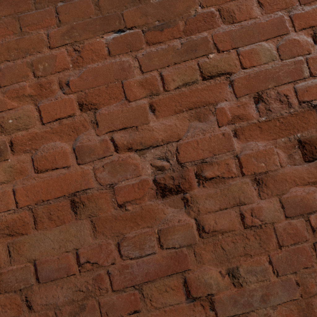
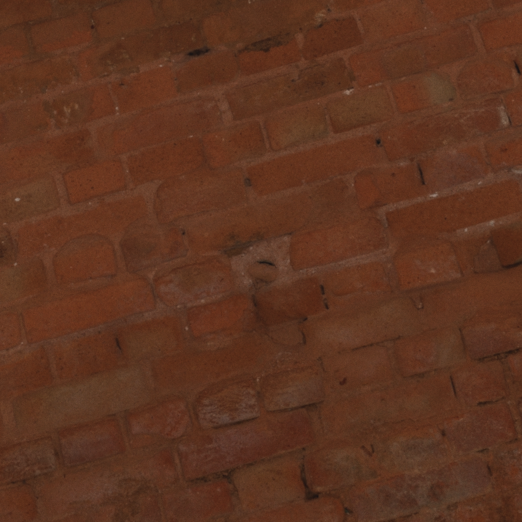
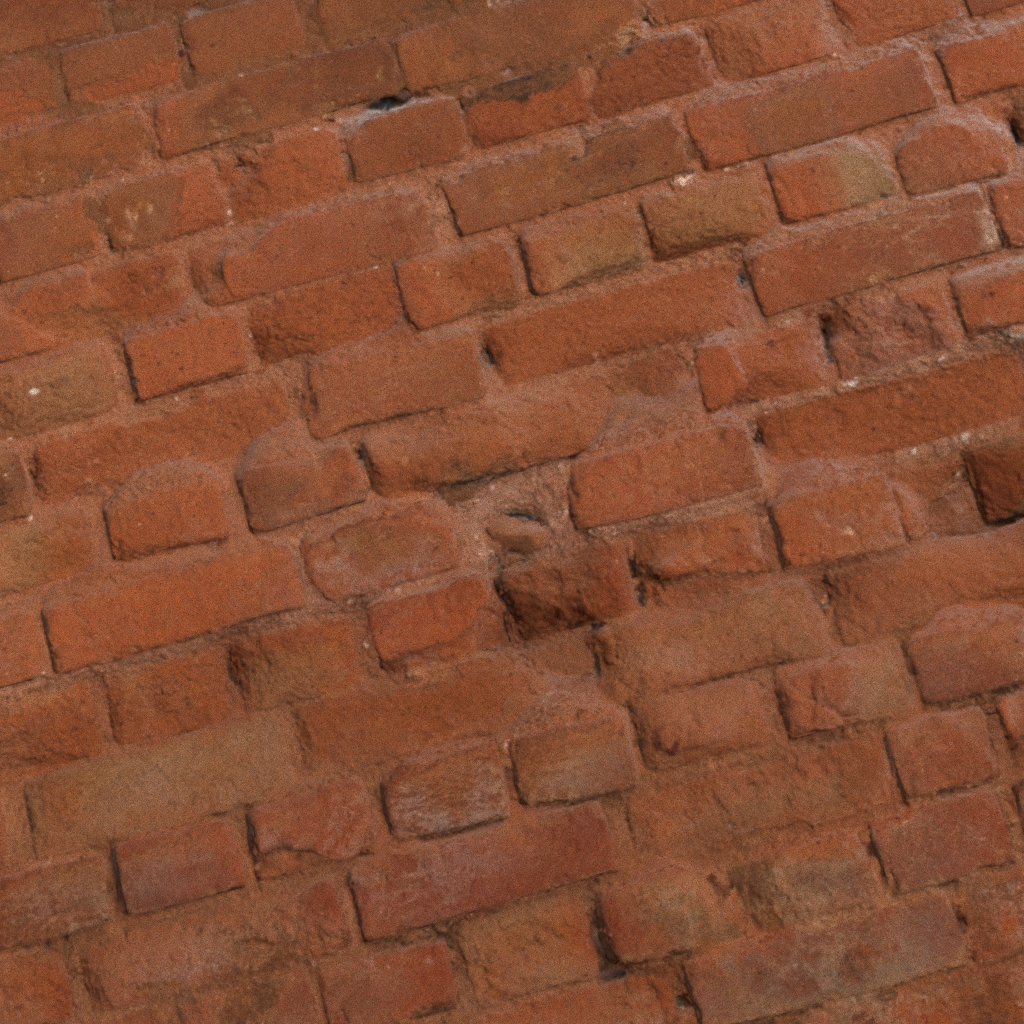
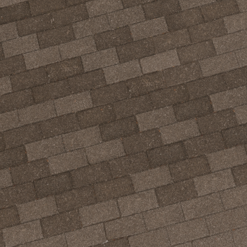
Adds per-pixel surface detail by perturbing the shading normal based on a normal map texture. This allows low-polygon meshes to appear highly detailed without additional geometry. Normal maps store encoded surface normal directions in RGB channels, which are transformed into the surface's tangent space and used for lighting calculations.
Implementation Summary
Modified Components:
src/core/instance.cpp - Normal map texture loading and application- Tangent space construction from surface geometry
- Normal map decoding from [0,1] to [-1,1] range
- Transform from tangent space to world space
- Orthonormal frame maintenance for consistency
Implementation Details:
- Construct tangent frame from surface normal and UV gradients
- Sample normal map texture at intersection UV coordinates
- Decode RGB → XYZ normal:
normal = 2.0 * rgb - 1.0
- Transform normal from tangent space to world space
- Normalize result and use for BSDF evaluation and light sampling
Biggest Challenge
Tangent Space Construction: The most challenging aspect was correctly constructing the tangent-bitangent-normal (TBN) frame for arbitrary meshes. Many meshes don't have pre-computed tangent vectors, requiring automatic generation from UV gradients. The challenge was handling degenerate cases:
- Triangles with zero or nearly-zero UV area (no texture gradient)
- Discontinuous UV seams where tangent frames flip
- Ensuring the TBN frame is orthonormal for correct lighting
- Handling normal map coordinate conventions (OpenGL vs DirectX)
- Maintaining consistent handedness across the mesh
The solution involved robust tangent frame generation with fallback cases and careful validation of the orthonormality of the resulting frame.
Alpha Masking / Transparency
Description
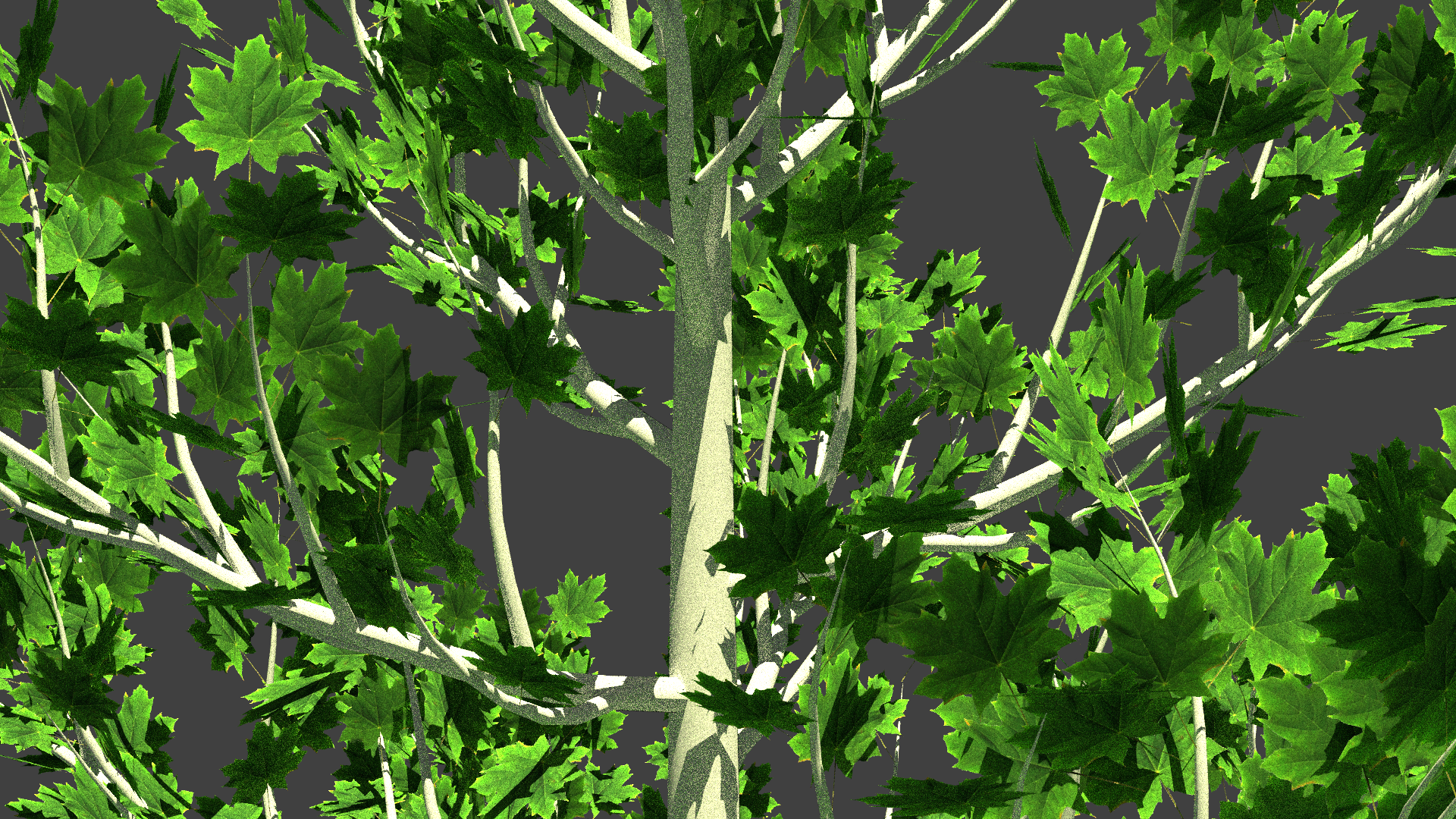
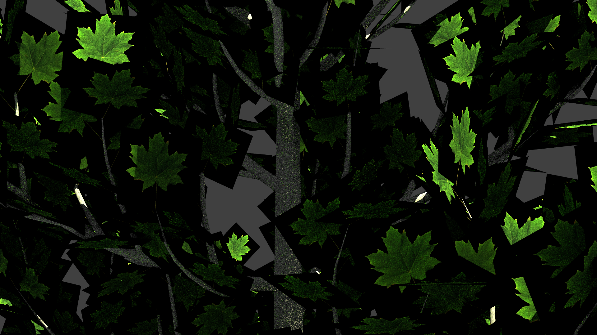
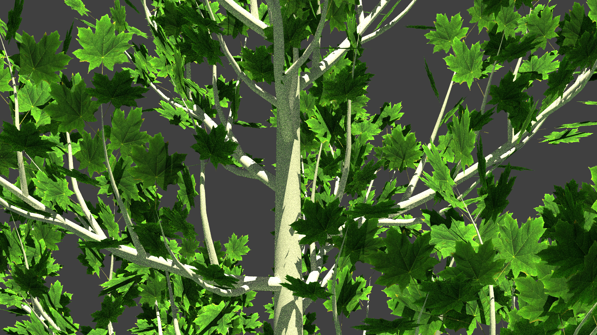
Implements stochastic alpha testing for rendering leaves, grass, and other objects with binary transparency. Rather than storing complex geometry for every leaf edge, alpha masking uses a texture's alpha channel to probabilistically accept or reject ray intersections. This creates the appearance of detailed cutouts from simple geometry.
Implementation Summary
Modified Components:
src/bsdfs/*.cpp - Added evaluateAlpha(uv) method to all BSDFssrc/core/instance.cpp - Alpha testing in intersection routine- Probabilistic ray continuation based on alpha value
- Importance sampling of alpha for variance reduction
Algorithm:
- Sample alpha value from texture at intersection UV
- Generate random number in [0,1]
- If random < alpha: accept intersection
- If random ≥ alpha: reject intersection, continue ray
- Bias compensation to maintain unbiased Monte Carlo estimator
Biggest Challenge
Self-Intersection and Ray Continuation: The biggest challenge was handling the case where a ray is rejected and needs to continue through the surface. Simply continuing the ray caused immediate re-intersection with the same surface (self-intersection), creating an infinite loop.
The solution required:
- Advancing the ray origin by a small epsilon offset
- Tracking ray depth to prevent infinite recursion
- Properly handling the case of multiple overlapping transparent surfaces
- Maintaining correct PDF and weight accounting for unbiased rendering
- Testing with complex scenes (trees, grass) to verify correctness
Solid Geometry
Alpha Masked Leaves
Credits & Resources
This project would not have been possible without the generous contributions of the 3D modeling community and various educational resources. Below, we acknowledge all the assets, tools, and references that helped bring "The Last Stand" to life.
Tools & Software
- Blender - 3D modeling, scene composition, and export
- Mixamo - Character rigging and animation poses
- Lightwave Renderer - Custom ray tracing engine (developed for this project)
- VS Code - Code development environment
- Git - Version control
- tev - HDR image viewer for render preview
Learning Resources & References
- Physically Based Rendering: From Theory to Implementation - Matt Pharr, Wenzel Jakob, and Greg Humphreys (pbrt.org)
- Computer Graphics Course Materials - Saarland University, Winter Semester 2025/26
- SIGGRAPH Papers - Various rendering and sampling techniques
- Sobol Sequence Implementation - Joe and Kuo direction numbers
- GGX/Microfacet BRDF Papers - Walter et al., Heitz et al.
Special Thanks
- Course Instructors & TAs - For guidance and support throughout the project
- Lightwave Framework Contributors - For providing the base rendering framework
- Open Source Community - For tools like Blender, stb_image, tinyexr, and more
- 3D Artist Community - For sharing high-quality models and assets
Disclaimer: Star Wars, its characters, and related elements are trademarks and copyrights of Lucasfilm Ltd. and The Walt Disney Company. This project is a non-commercial academic work created for educational purposes only. All assets were used in accordance with their respective licenses and terms of use.