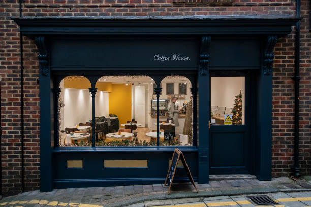
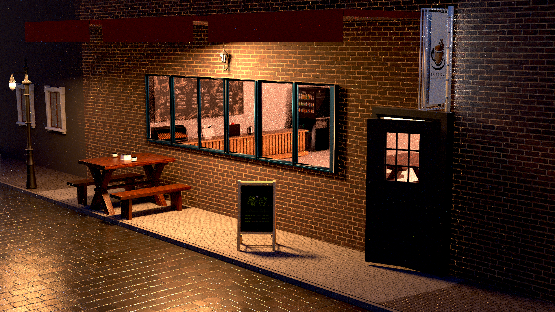
Final Render - "The Midnight Grind"

Motivation

We wanted to move away from pristine, daylight architectural visualization and instead capture a "lived-in" but empty at night urban mood.

Artistic Intention

The scene tells the story of a quiet refuge in a sleepy city. It is meant to evoke a feeling of coziness that is contrasted against the solitude of a dark street. The warm orange and yellow hues of the interior and the street lämp are designed to battle the darkness, inviting the viewer to step inside out of the cold. It captures that specific moment late at night when the streets are empty, but life still hums quietly behind the glass.

Technical Details

  • Render Time: 2 minutes @ 128 samples

Hardware Used:

  • GPU: NVIDIA RTX 3060
  • CPU: AMD Ryzen 7 5800X3D
  • RAM: 128GB DDR4

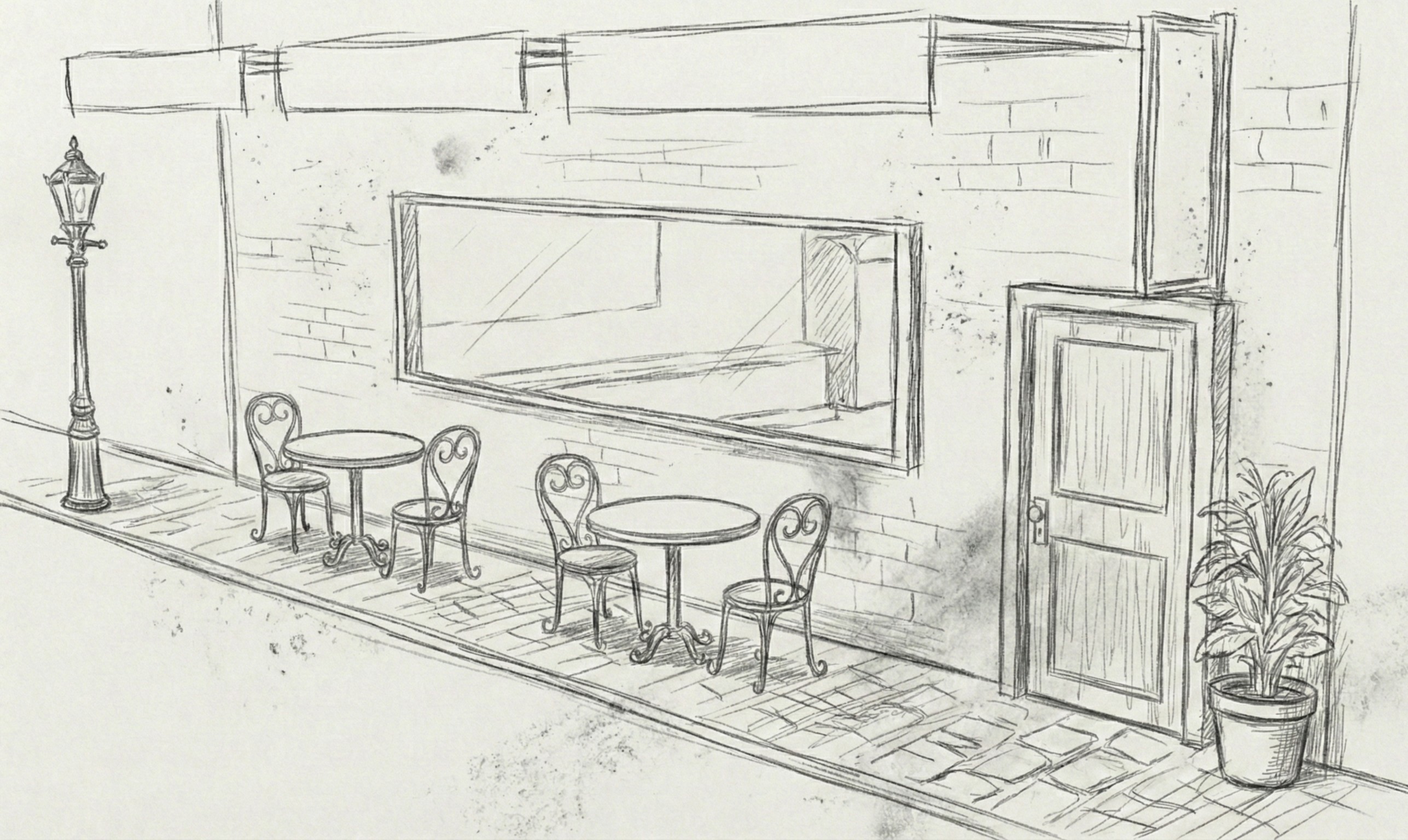
Why does it look different from the sketch?

Bcs we didn't wanna pay for the blender assets therefore we recreated it with what we had for free *shrugs*

What we have used:

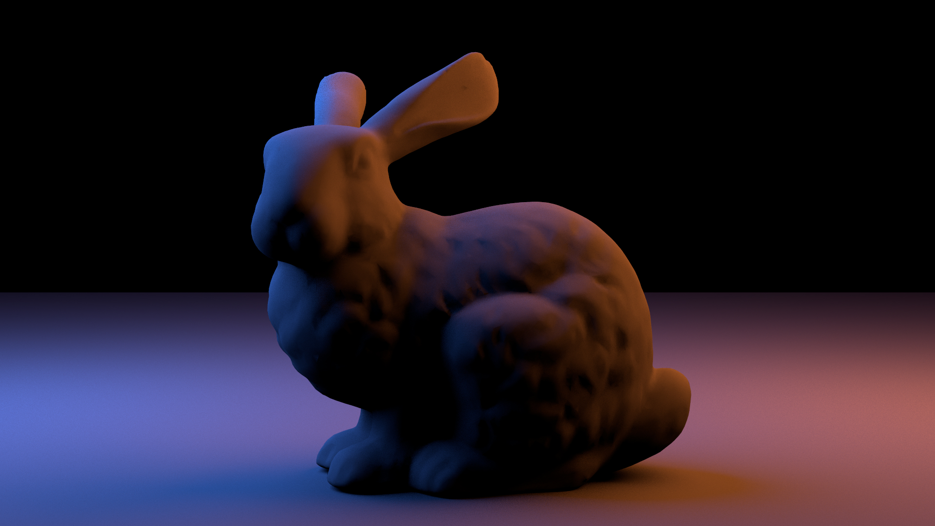
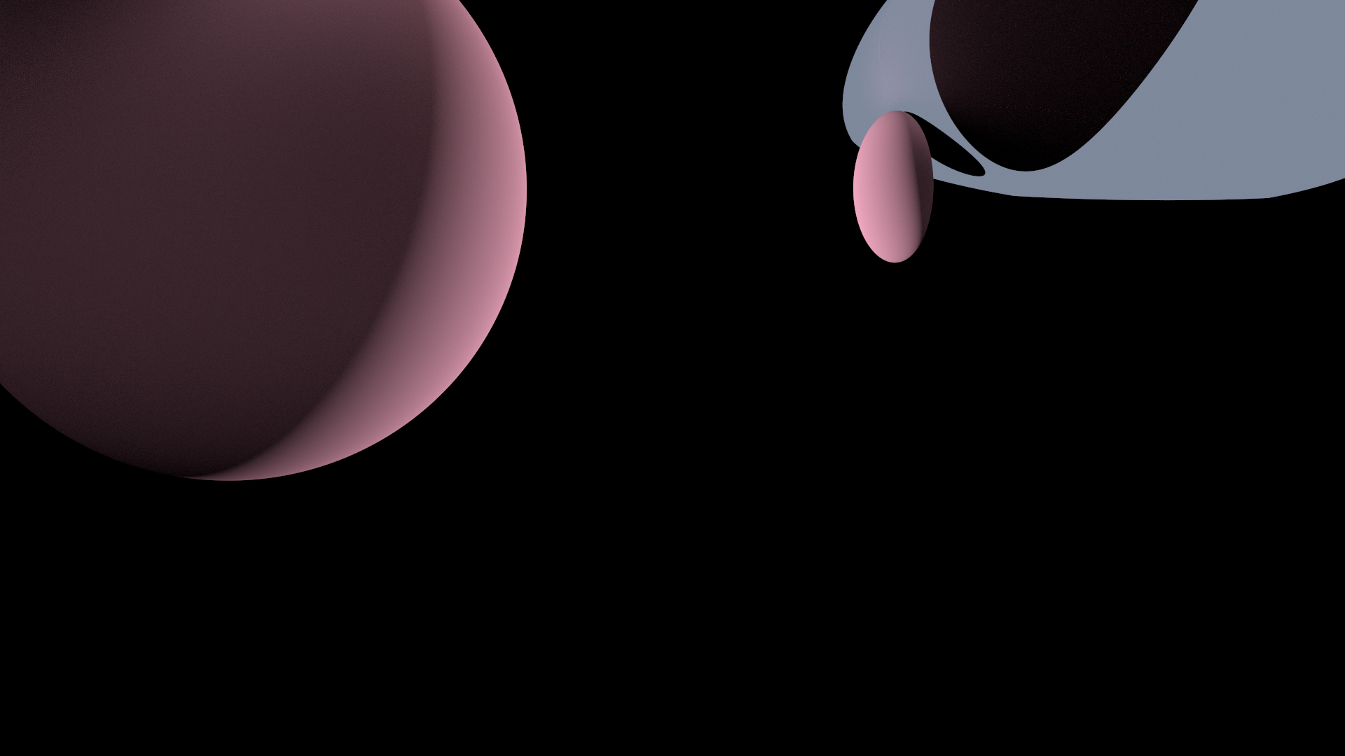
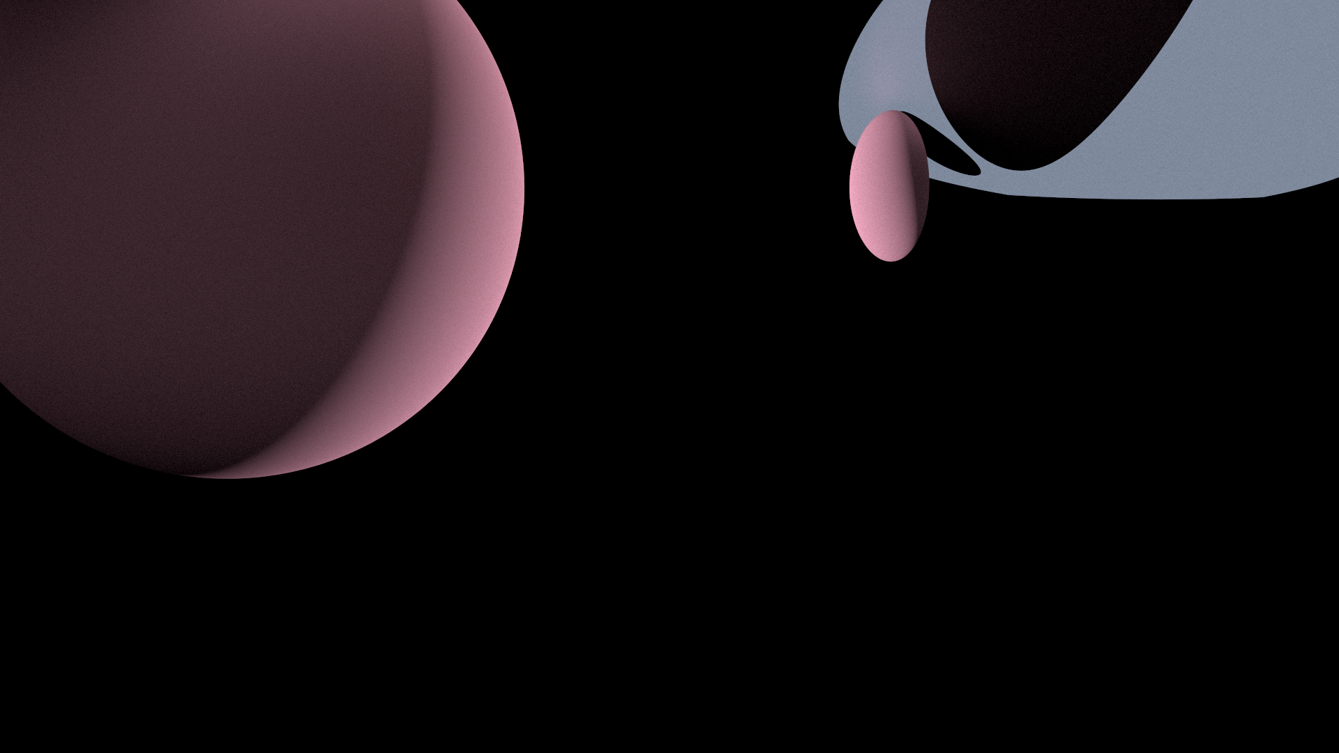
Area Lights

Previously, a light source only contributed to the scene if it was by chance hit by a ray, so-called "implicit light sampling". With area lights, we can now sample points on the light source itself, leading to more accurate and realistic lighting in scenes. This is particularly noticeable in scenes with large light sources or when achieving soft shadows.

Implementation Details

The implementation involved moving from a passive light transport model to Next Event Estimation. We modified the following core components:

  • Implemented sampleArea for the Sphere primitive (sampling a uniform point on the surface)
  • Created a new sampling routine that, upon hitting a surface, selects a light source at random (proportional to its area) and picks a point P' on its surface.
  • Adjusted the radiance calculation to ensure that if a ray hits a light source "by accident", its contribution is ignored.

Challenges

One of the most significant challenges was the correct application of the weight formula.
In the sampleDirect method, we had to make sure that the contribution was correctly dampened by the squared distance (1/r^2) and the cosine of the angle at the light source.

Modified files

  • area.cpp | implemented area lights and next event estimation for realistic lighting.
  • sphere.cpp | implemented sampleArea method for uniform surface sampling on spheres.
After After
Before Before

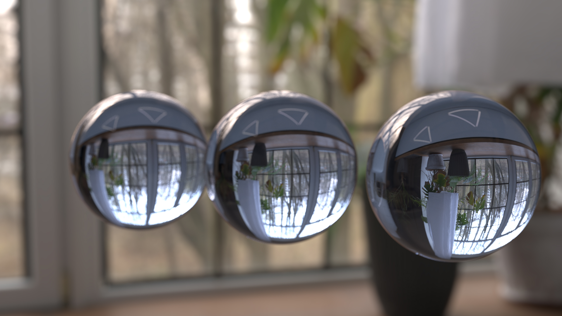
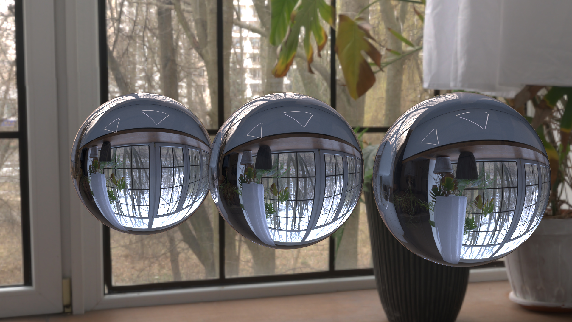
Thin Lens Camera

To introduce physical realism to our camera model, we implemented a Thin Lens Camera. Unlike a standard pinhole camera where every object in the scene is perfectly in focus, the thin lens model simulates the finite size of a real camera aperture. This enables Depth of Field (DoF) effects, where only objects at a specific focal distance appear sharp, while those closer or further away become progressively blurred.

Implementation Details

The implementation replaces the single point of origin used in pinhole cameras with a physical lens disk.

  • We use squareToUniformDiskConcentric to map random numbers to a uniform point on a circular lens.
  • For every pixel, we calculate a target point on the focal plane at z = focalDistance.
  • Instead of starting all rays from [0,0,0], each ray now starts from the sampled point on the lens. The direction is determined by the vector pointing from the lens sample to the focal point.
  • The resulting local ray is transformed into world space using the camera’s transformation matrix, allowing the camera to be positioned and oriented anywhere in the scene.

Challenges

The most challenging aspect of this feature was correctly calculating the focal point coordinates in relation to the field of view (FoV). Specifically, when the aperture radius is non-zero, the ray origin is shifted. If the focal point isn't calculated proportionally to the focalDistance using the tan(halfFov), the resulting image will suffer from shift in the field of view and incorrect magnification.

Modified files

  • thinlens.cpp | implemented the thin lens camera model and depth of field effects.
After After
Before Before

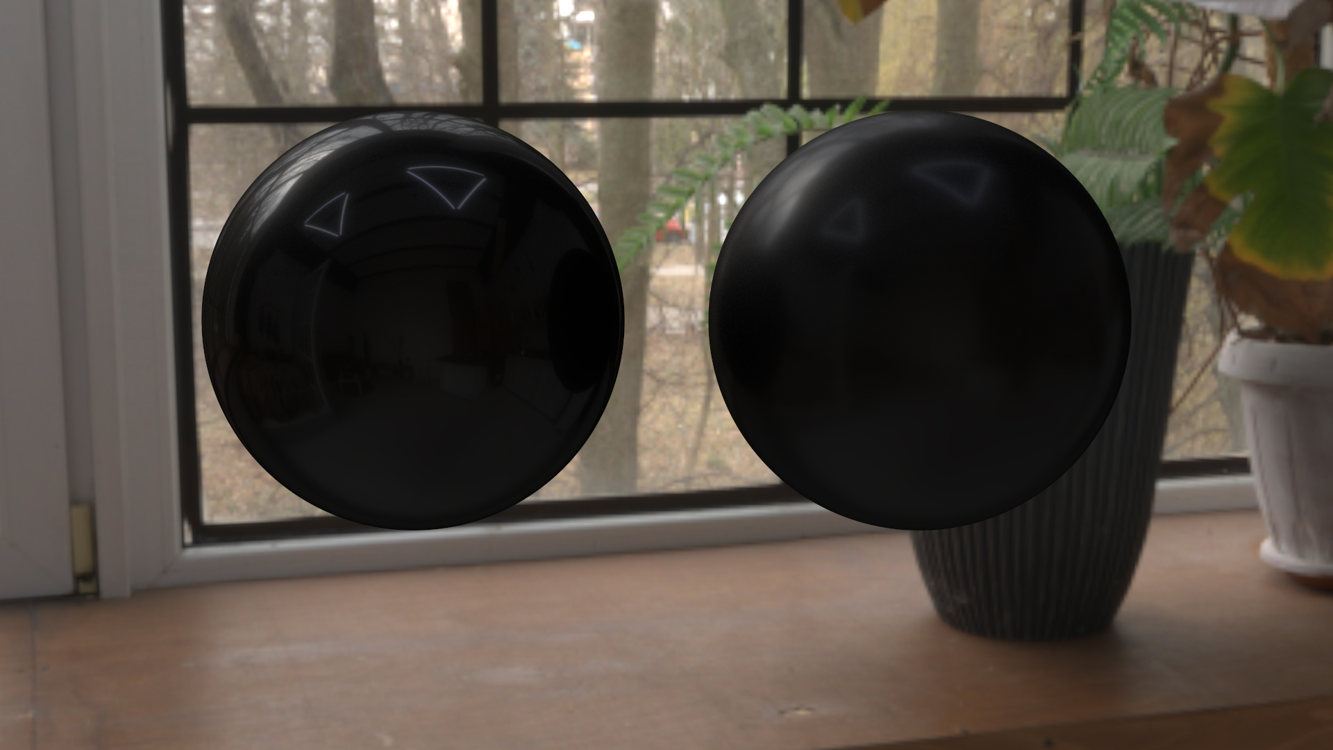
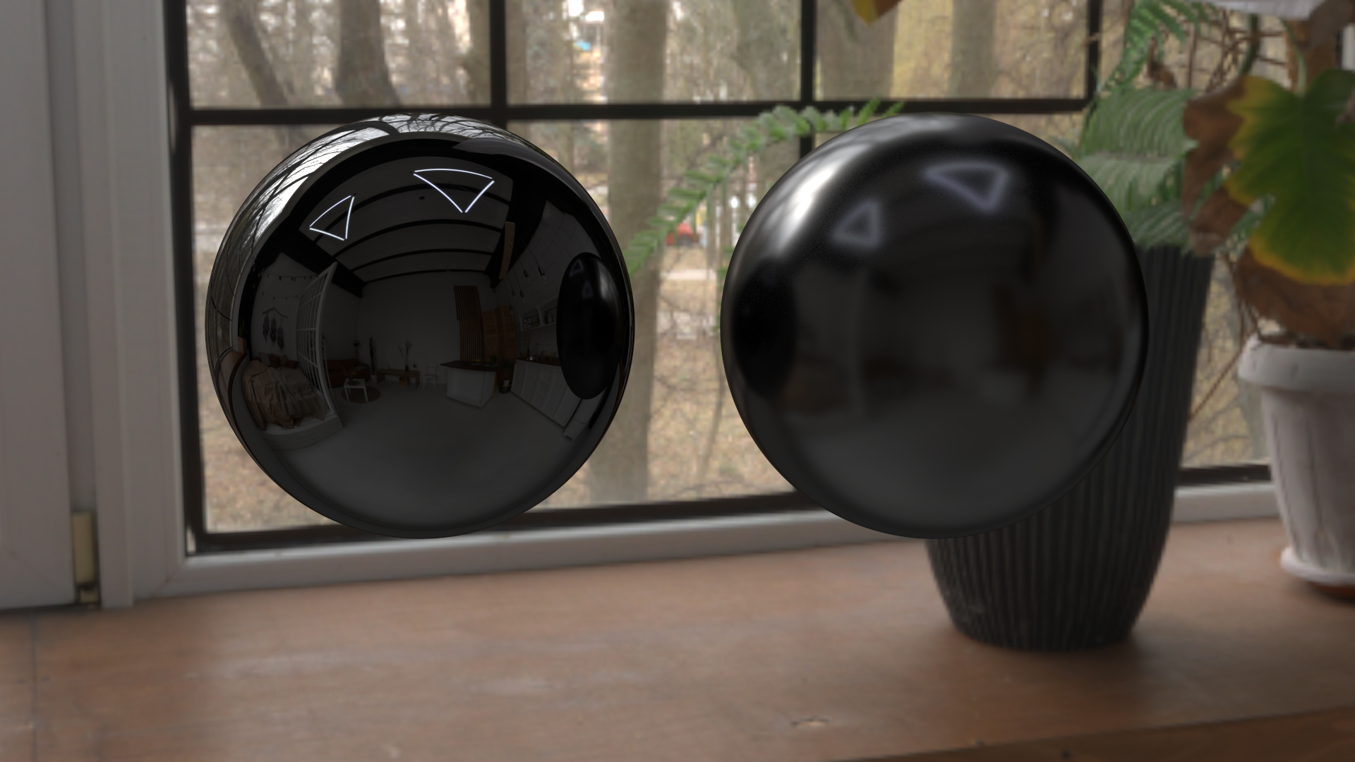
Clearcoat Material

Standard materials often assume light interacts with only a single surface layer. However, many real-world materials—like car paint, polished wood, or gloss-coated plastics—feature a diffuse base covered by a translucent, reflective top layer. We implemented a Clearcoat BSDF to simulate this multi-layered appearance, adding a distinct "polish" and secondary specular highlights to our objects.

Implementation Details

The clearcoat layer is modeled as a high-gloss specular layer sitting atop a diffuse base. The implementation uses several sophisticated statistical models to ensure physical accuracy:

  • GTR1 Distribution: We implemented the Berry (GTR1) microfacet distribution for the clearcoat highlights, which provides a longer "tail" than standard GGX, resulting in a more realistic soft glow around sharp reflections.
  • Layered Reflection/Refraction: The BSDF uses the Schlick approximation of Fresnel terms to dynamically balance energy between the clearcoat reflection and the base diffuse layer.
  • Importance Sampling: To maintain high performance, we implemented a stochastic sampling strategy. The renderer chooses between sampling the clearcoat (via GTR1 distribution) or the diffuse base (via cosine-weighted hemisphere sampling) based on their relative luminances.
  • Geometric Masking: We utilized a separable Smith GGX shadowing-masking term G1 to account for microfacet self-shadowing at grazing angles.

Challenges

The primary challenge was implementing Importance Sampling for the GTR1 distribution. Unlike standard diffuse materials, the GTR1 distribution has a very specific mathematical "tail" that requires a complex Inverse Cumulative Distribution Function (Inverse CDF) to sample correctly. Ensuring the PDF (Probability Density Function) perfectly matched the distribution was critical; even a slight mismatch resulted in "fireflies" or darkened edges on spheres.

Modified files

  • clearcoat.cpp | Implemented the GTR1 distribution, Smith masking, and layered BSDF logic.
  • fresnel.hpp | Utilized Schlick's approximation for efficient energy layering.
After After
Before Before

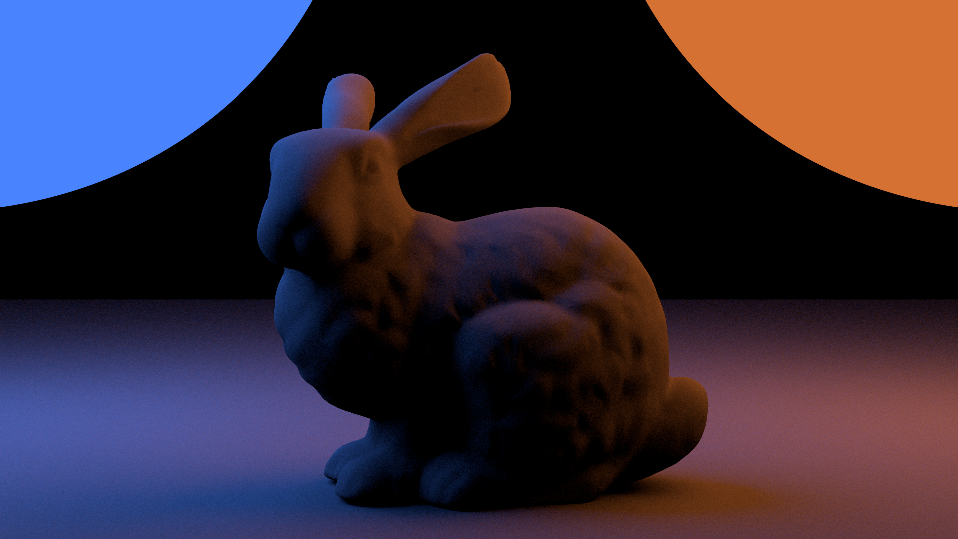
Improved Environment Sampling

High Dynamic Range (HDR) environment maps are essential for realistic lighting, but they often contain concentrated areas of high intensity, such as the sun. In our initial implementation, the background was only sampled when a ray happened to exit the scene. By adding Next Event Estimation support for the environment, we can now actively sample the background, dramatically reducing noise and enabling sharp shadows from distant light sources.

Implementation Details

To efficiently sample the environment, we implemented a Hierarchical Importance Sampling scheme that prioritizes bright pixels (high energy) in the HDR map:

  • 2D Distribution Mapping: We pre-calculate a 2D PDF based on the luminance of the texture. This is achieved by creating a marginal distribution for the rows (V) and multiple conditional distributions for the columns (U).
  • Spherical Compensation: When building the luminance map, we scale each pixel by sin(theta). This compensates for the distortion inherent in equirectangular projections, preventing over-sampling at the poles.
  • CDF Inversion Sampling: Using std::upper_bound, we perform a binary search on the Cumulative Distribution Function (CDF). This allows us to transform a uniform random number into a sample that perfectly matches the energy distribution of the environment.
  • PDF Conversion: Since the importance sampling is performed in UV/Area space, we convert the PDF to solid angle measure using:
    PDFω = PDFuv / (2π2 ⋅ sinθ)

Challenges

Debugging the PDF conversion was time-consuming; if the sin(theta) term is not handled carefully at the poles (where it approaches zero), it causes numerical instability and "black pixels" in the final render.

Modified files

  • envmap.cpp | Implemented 1D and 2D Distributions and integrated sampleDirect.
After After
Before Before

Low-Discrepancy Sampler (Halton)

In Monte Carlo rendering, the quality of the image depends heavily on how uniformly random samples are distributed across the integration space. Standard "independent" samplers often produce clusters of points or large empty gaps, leading to visible noise. To address this, we implemented a Halton Sampler, a quasi-random sequence designed to maintain low discrepancy—ensuring that samples are well-distributed and "stratified" across any number of dimensions.

Implementation Details

The Halton sequence generates points by utilizing the Radical Inverse function in different prime bases. Our implementation includes several advanced features:

  • Multi-Dimensional Stratification: Each dimension of the sampling problem (e.g., pixel X, pixel Y, lens position, light surface) is assigned a unique prime number as its base (2, 3, 5, 7, etc.). This ensures that samples are decorrelated across different integration domains.
  • Scrambled Radical Inverse: To prevent structural patterns (aliasing) that can occur in vanilla Halton sequences, we implemented scrambling. By applying a permutation based on the pixel coordinates (using the FNV-1a hash), we shift the sequence differently for every pixel.
  • Incremental Dimension Tracking: The sampler maintains a baseIndex that automatically increments with every call to next(), ensuring that each subsequent random number queried during a single path belongs to a new, well-distributed dimension.

Challenges

The biggest challenge was achieving proper pixel decorrelation. In a basic Halton sequence, neighboring pixels can often receive very similar sample values, which manifests as distracting structural artifacts or "grid-like" patterns in the final render.

We overcame this by implementing a pixel-dependent scrambling logic. Debugging this required visualizing the 2D distribution of samples to ensure that while each pixel's samples were uniformly distributed, the specific pattern changed from one pixel to the next. Ensuring the radicalInverse function remained numerically stable and efficient while handling high sample indices and various prime bases was also a key technical hurdle.

Modified files

  • halton.cpp | Implemented the scrambled radical inverse and the Halton sequence sampler.
After After
Before Before

Normal Mapping

Normal Mapping

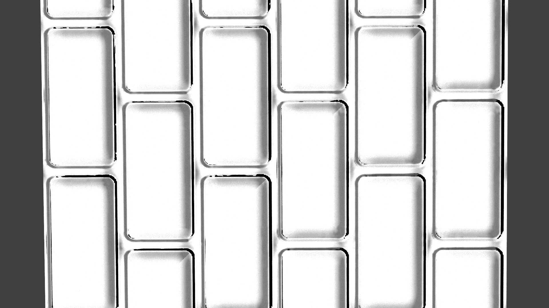
To achieve high levels of visual detail without significantly increasing geometric complexity, we implemented Normal Mapping. This technique allows us to simulate intricate surface features—such as scratches, pores, or embossed patterns—by perturbing the surface normal used in lighting calculations. By faking the way light bounces off a surface, we can make a simple flat plane appear as though it has complex, three-dimensional depth.

Implementation Details

Normal mapping was integrated directly into the Instance::transformFrame method, ensuring that all shapes—regardless of their primitive type—automatically support this feature.

  • Tangent Space Transformation: Normal maps are stored in "tangent space" (the local coordinate system of the surface). We use the surface's tangent, bitangent, and shading normal to build a coordinate frame that transforms the sampled normal into world space.
  • Data Remapping: Since color textures store values from [0, 1] but surface normals exist in the range [-1, 1], we apply a remapping formula: n = 2 ⋅ color - 1.
  • Dynamic Perturbation: The shadingNormal of the SurfaceEvent is updated using the sampled normal, while the geometryNormal remains unchanged. This ensures that shading is detailed while ray-object intersections remain computationally efficient.

Challenges

The primary challenge was ensuring the orthonormal consistency of the shading frame after transformations were applied.

When an object is scaled or rotated via the m_transform, the tangent and normal must be transformed correctly before the normal map is applied. If the transformation or the subsequent reconstruction of the normal in world space is off by even a small degree, the lighting will appear to "flip" or look inverted as the camera moves around the object. Correcting the vector math to ensure the normal was reconstructed in the correct Tangent-Bitangent-Normal order.

Modified files

  • instance.hpp | Added the m_normal texture property to the Instance class.
  • instance.cpp | Implemented the normal remapping and tangent space reconstruction logic.
After After
Before Before

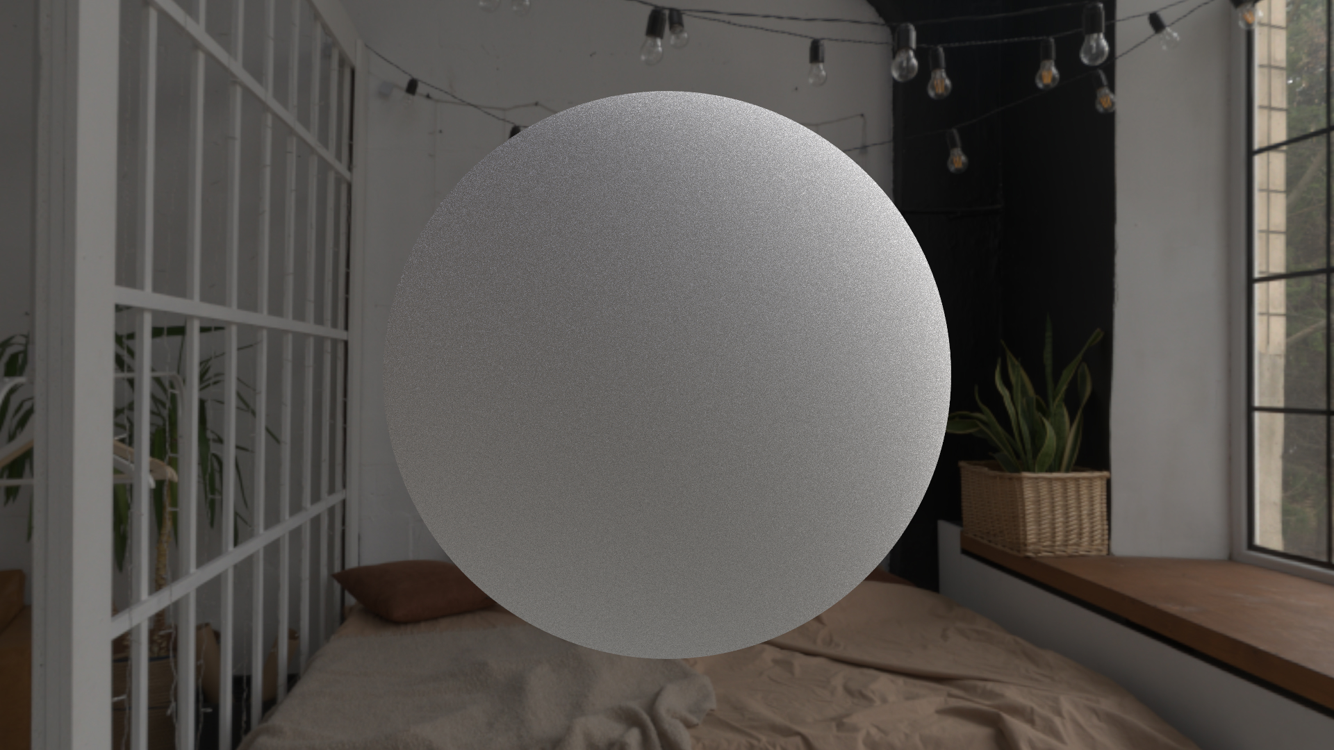
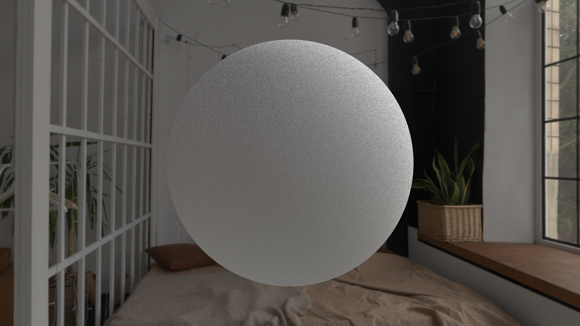
Rough Dielectric

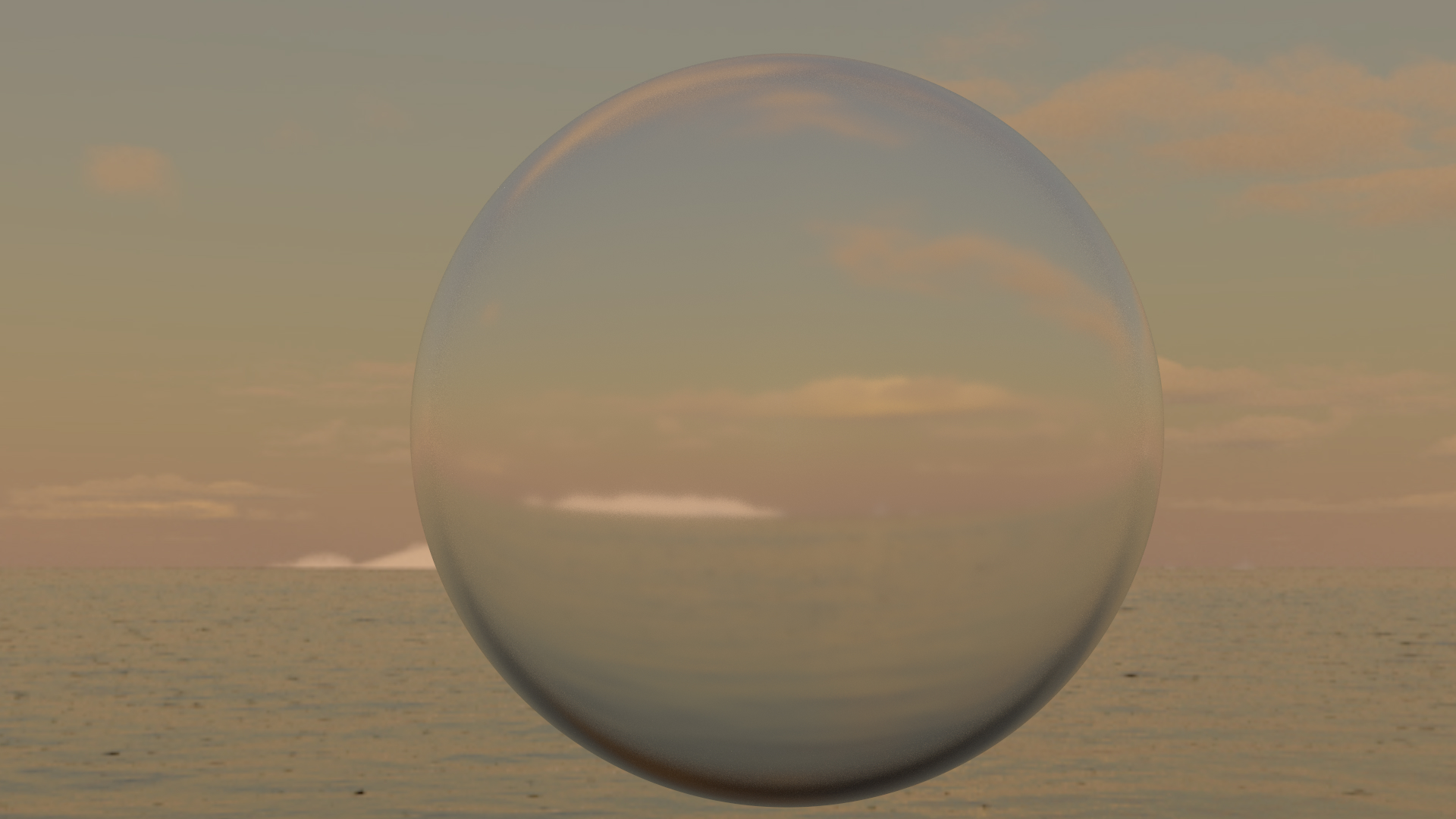
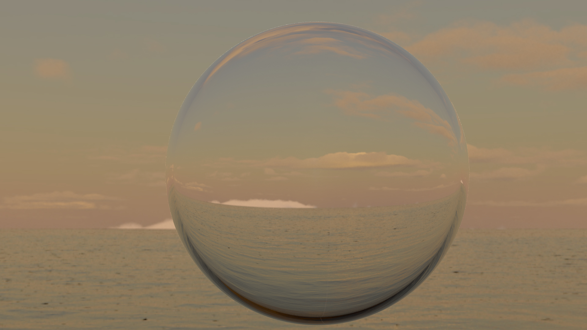
While standard dielectrics simulate perfectly smooth surfaces like glass or water, real-world transparent materials often possess microscopic surface irregularities. We implemented the Rough Dielectric BSDF to simulate these materials, enabling effects like frosted glass, etched crystals, or rough plastic. This model accounts for light being both reflected and refracted through a surface covered in microscopic "facets," scattering light into a soft glow.

Implementation Details

This feature combines microfacet theory with Snell's law and Fresnel equations to create a physically grounded model for translucent scattering:

  • GGX VNDF Sampling: To achieve high efficiency, we utilized Visible Normal Distribution Function (VNDF) sampling. This selects microfacet normals (wh) that are specifically visible from the view direction, significantly reducing noise compared to standard NDF sampling.
  • Energy-Balanced Stochastic Sampling: The BSDF uses the Fresnel coefficient to stochastically decide whether a ray should reflect off the surface or refract through it. This ensures that the material remains energy-neutral and physically accurate.
  • Refractive Jacobian: Unlike reflection, refraction involves a change in the medium's Index of Refraction (IOR). We implemented a scaling factor based on the relative IOR ($1/\eta^2$) to correctly account for the compression of radiance across different media.
  • Smith G1 Masking: We integrated the Smith shadowing-masking function to model how microfacets obscure one another at grazing angles, preventing the material from appearing unnaturally bright at the edges.

Challenges

The most difficult aspect of this implementation was handling the refractive half-vector transformation.

In a rough conductor (reflection only), the relationship between the half-vector and the incoming ray is straightforward. However, in refraction, the "half-vector" calculation depends on the ratio of the Indices of Refraction ($\eta$). Correcting the weight calculation to include the specific Jacobian of the refraction transformation—while ensuring that total internal reflection (TIR) and rays entering/exiting different hemispheres were correctly handled—was mathematically intensive. A single sign error in the IOR ratio or the dot products would lead to energy leaks or "black" regions in the refractive highlights.

Modified files

  • roughdielectric.cpp | Implemented GGX VNDF sampling and the refractive microfacet model.
  • microfacet.hpp | Utilized Smith G1 and GGX distribution functions.
After After (Roughness 0.2)
Before Before (Roughness 0.0)