Bloom
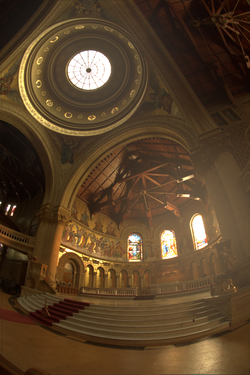
Bloom is a post-processing effect that simulates the optical scattering of light within a camera lens or the human eye. It causes bright light sources to bleed or "glow" beyond their physical boundaries, enhancing the perceived dynamic range and realism of the image by signaling brightness levels that exceed the monitor's display capabilities.
Pipeline & Thresholding:
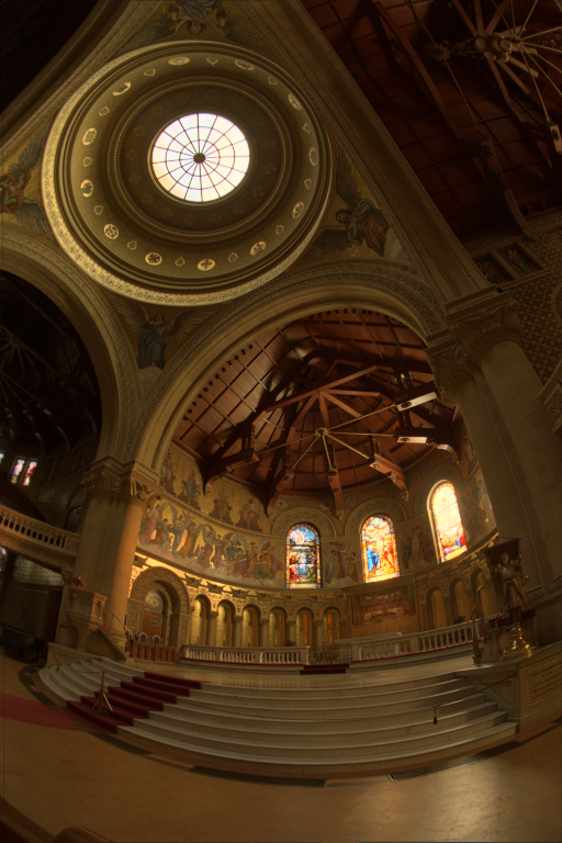
The effect is implemented in a dedicated Bloom post-processing class. The pipeline first extracts high-intensity pixels by filtering the original image against a luminance threshold. This isolates the "bright" regions that are intended to glow.
Separable Gaussian Blur:
The core glow effect is created by applying a Gaussian blur to the extracted highlights. To ensure performance, I utilized a separable kernel optimization. Instead of performing a computationally expensive 2D convolution (scaling with \(O(k^2)\) per pixel), I decomposed the operation into two sequential 1D convolutions (horizontal and vertical, scaling with \(O(2k)\) per pixel).
Compositing:
Finally, the blurred highlight map is additively combined with the original rendered image to produce the final result.
Bloom Effect
 No Bloom Effect
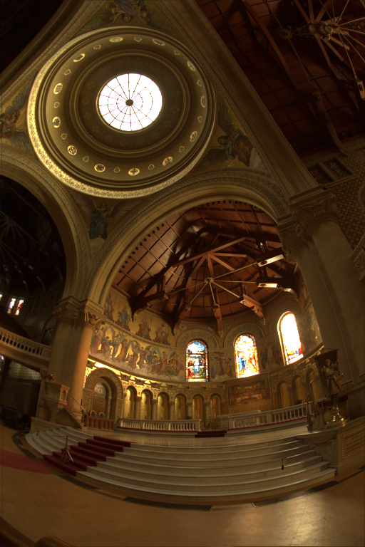
No Bloom Effect
Attributions
- Image: Stanford memorial church
The implementation was straightforward and proceeded without significant difficulties. The separable convolution algorithm is well-documented, and integrating the multi-pass structure (threshold, blur, combine) into the post-processing pipeline worked as expected.
Luminance Tone Mapping
The basic Reinhard operator implemented during the assignments operates on each RGB channel independently. While simple, this approach causes color shifts and desaturation because the ratios between color channels change non-uniformly.
Luminance Tone Mapping solves this by calculating the perceived brightness (luminance) of a pixel, compressing that scalar value, and then scaling the original RGB color vector. This preserves the chromaticity and saturation of the original image, ensuring that colors remain vibrant even after compression.
Luminance (\(Y\)) is calculated based on human visual sensitivity:
\[ Y = 0.2126 \cdot R + 0.7152 \cdot G + 0.0722 \cdot B \]
Modes & Architecture:
I extended the existing ToneMapping class to support a configurable mode via an enum parameter. This allows switching between four distinct behaviors:
- Reinhard (RGB): Standard per-channel compression.
- Reinhard (Luminance): Preserves color ratios using the luminance formula.
- Extended Reinhard (RGB): Allows white-point control per channel.
- Extended Reinhard (Luminance): The most robust method, combining white-point control with chromaticity preservation.
Extended Operator:
The "Extended" variant introduces a white point parameter \(L_{white}\), which defines the luminance value that should map to pure white (1.0). This prevents the image from looking "flat" by allowing very bright highlights to burn out naturally:
\[ L_{out} = \frac{L_{in} (1 + \frac{L_{in}}{L_{white}^2})}{1 + L_{in}} \]
Memorial Church Comparison
Luminance Extended Reinhard (Best balance of contrast and saturation)
Luminance Reinhard
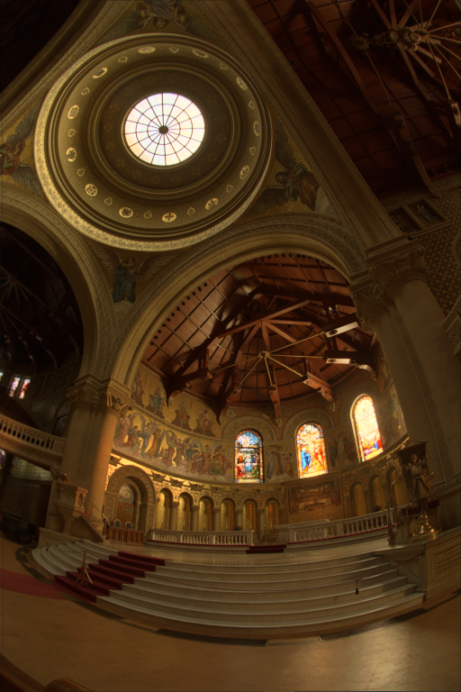 Extended Reinhard (RGB)
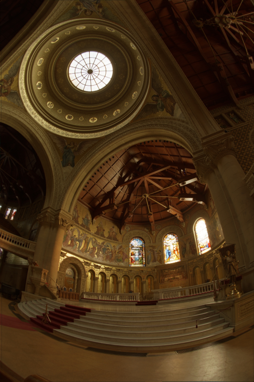 Reinhard (RGB) - Note the slight desaturation compared to Luminance versions
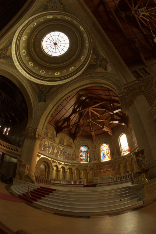 No Tonemapping (Clamping RGB values) - Notice the blown-out highlights and lack of detail
Attributions
- Image: Stanford memorial church
This feature was straightforward to implement, as it primarily involved extending the mathematical operators already present in the base assignment framework to support vector scaling based on the luminance scalar.
Denoising (OIDN)
To further reduce noise in the final render, this feature integrates the Open Image Denoise (OIDN) library as a post-processing step. The feature utilizes auxiliary AOVs (albedo and normal) to guide the denoising process, preserving important details while effectively reducing noise.
Integration:
The implementation is encapsulated within the DenoiserPostProcess class. The core functionality involves loading the library and utilizing the API to configure the denoiser with the rendered image and auxiliary buffers.
Auxiliary AOVs:
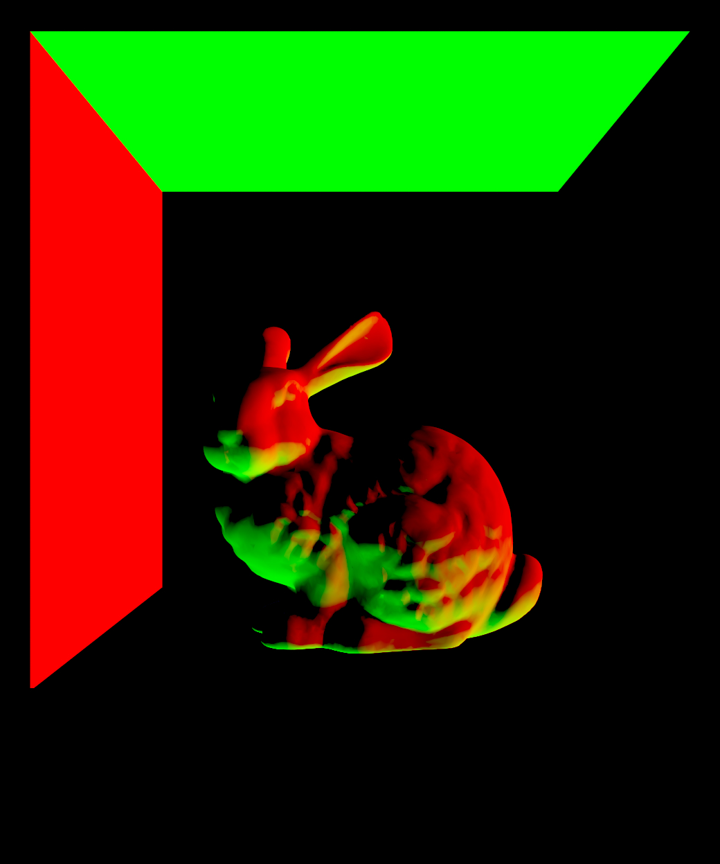
Correctly implementing the auxiliary AOVs was crucial. The library requires Albedo values to be in the \([0, 1]\) range, while Normals must be provided in World Space.
The Albedo query specifically required multiple iterations. I realized that for OIDN to work correctly with delta BSDFs (like glass), the albedo calculation needed to utilize the fresnel term. This necessitated modifying the texture query function to accept a wo (outgoing direction) vector.
Bunninator Scene
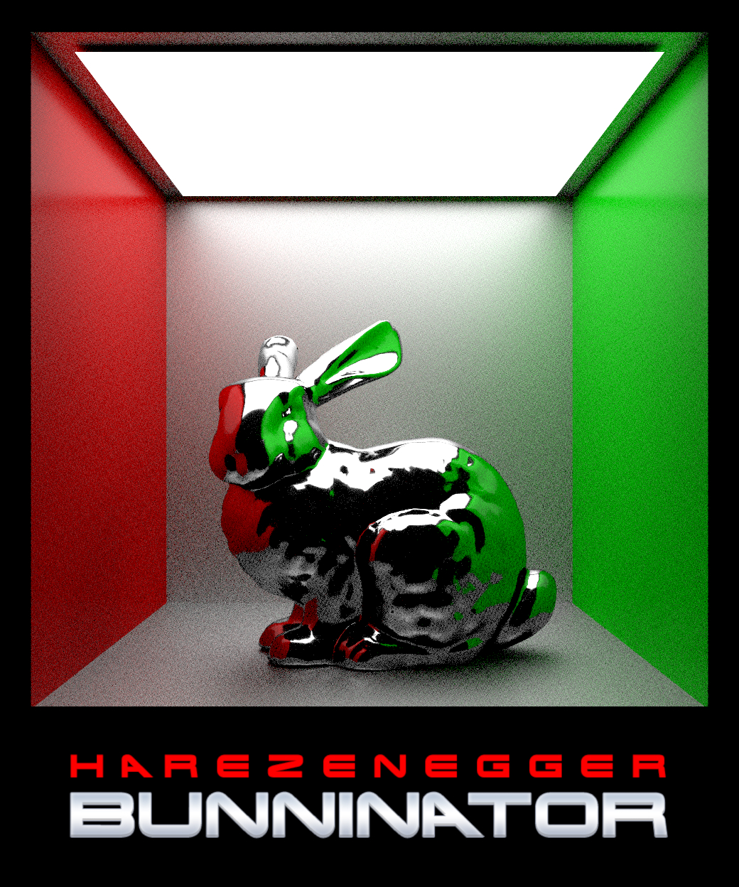
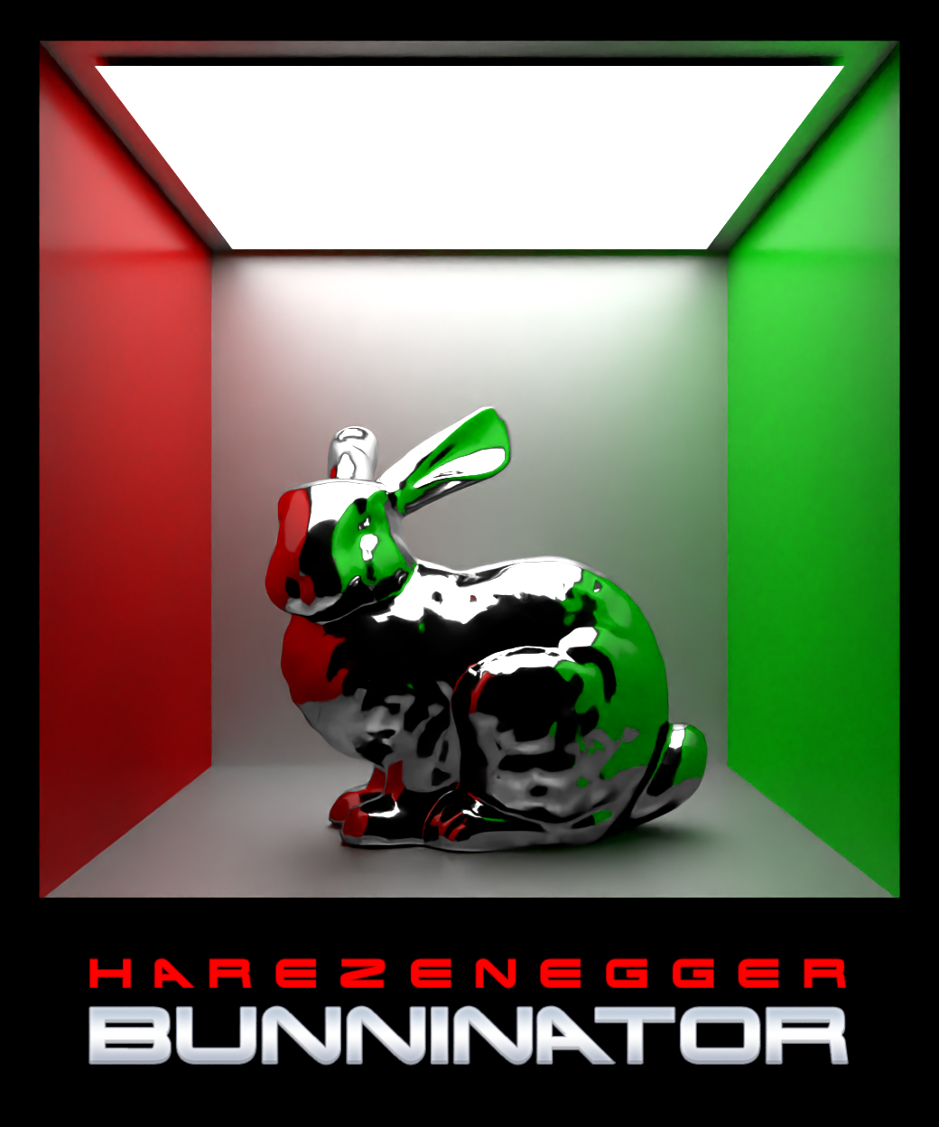
The denoiser can also help showcase the benefits of low-discrepancy sampling. Denoised Output (OIDN) with Halton Sampling with Owen Scrambling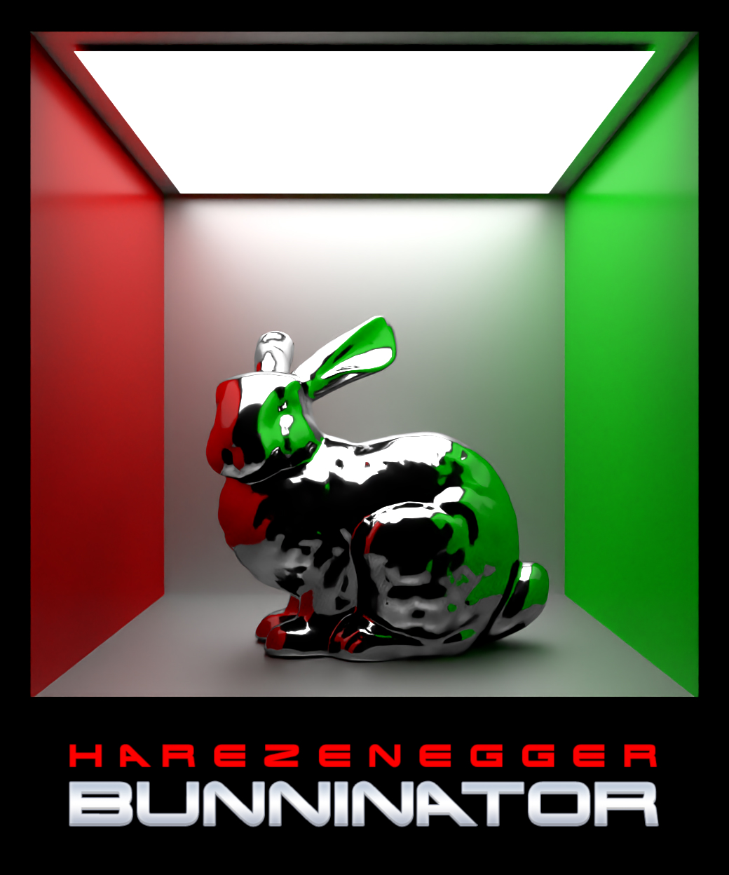 Raw Output (Noisy) with Halton Sampling with Owen Scrambling
 Denoised Output (OIDN) with Halton Sampling with no Scrambling.
Note the geometric patterns still visible in the denoised output due to the correlation of the samples.
Denoised Output (OIDN) with Halton Sampling with no Scrambling.
Note the geometric patterns still visible in the denoised output due to the correlation of the samples.
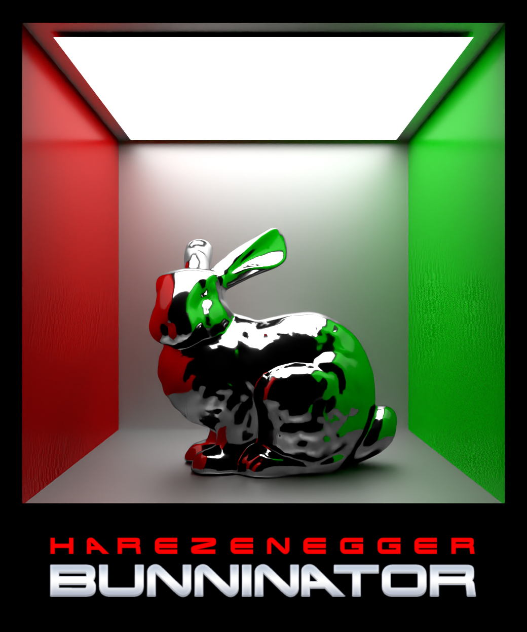 Raw Output (Noisy) with Halton Sampling with no Scrambling
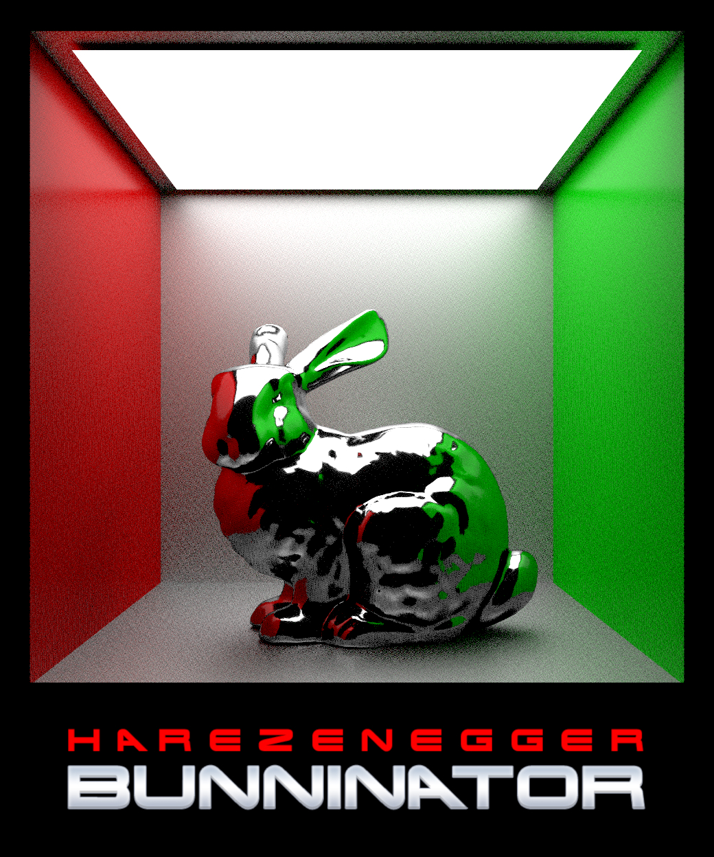 Denoised Output (OIDN) with independent sampling
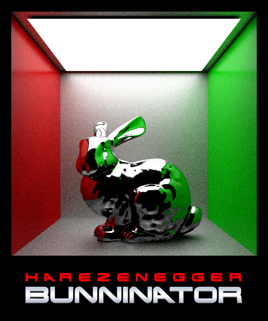
Note the higher noise on the ceiling and walls close to the light source.
Denoised Output (OIDN) with independent sampling
Note the higher noise on the ceiling and walls close to the light source.
 Raw Output (Noisy) with independent sampling
 Albedo AOV used for Denoising
 Normal AOV used for Denoising (World Space, so the clipping causes the negative values to be black)
A major challenge was configuring the GitLab CI to build the project. Since I couldn't get the CI to install dependencies automatically, I had to include the Linux library files directly in the repository to allow the tests to compile and run.
Implementing the correct AOVs presented several issues:
- The initial Albedo implementation failed for delta BSDFs because it lacked the
woterm required to calculate the fresnel component. - The default Normal AOV implementation from the assignments remapped values to \([0, 1)\), which is explicitly incorrect for OIDN; it requires raw world-space normals.
- Defining a "base color" for transparent materials and volumes for the Albedo AOV was ambiguous and difficult to define.
I initially wasted time considering if I needed to extend the integrator to correlate the color image samples with the AOV samples. I eventually realized that because the renderer uses deterministic sampling, the correlation is maintained automatically.