Intro
Inspiration
Our very different cultural background and our love for fiction, literature and visual arts gave us the initial spark of inspiration for this project. A shared fascination for magical realism and the way that it has shaped our understanding of the world led our imagination. Our goal was simple, to take a space that felt tangible, rooted in reality, mundane even, and then infuse it with the fantasy and magic that is only possible in fiction. One of the best examples of this kind of magical realism in recent memory is Mexican director (who funnily enough shares a name with both of us) Alejandro González Iñárritu's 2022 film "Bardo, False Chronicle of a Handful of Truths". In the first act of the movie, the main character rides a very unique subway car filled with water and inhabited by a family of Axolotls. This was the jumping off point for us, and almost immediately, this idea brought to mind another (un)familiar space. In a blissfully surreal scene of Hayao Miyazaki's "Spirited Away" our main character gets on a train that inexplicably rides across the ocean. In the background, nothing but clouds, the horizon and a warm sunset.
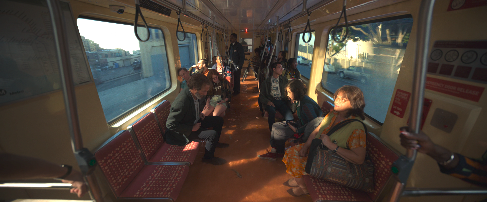
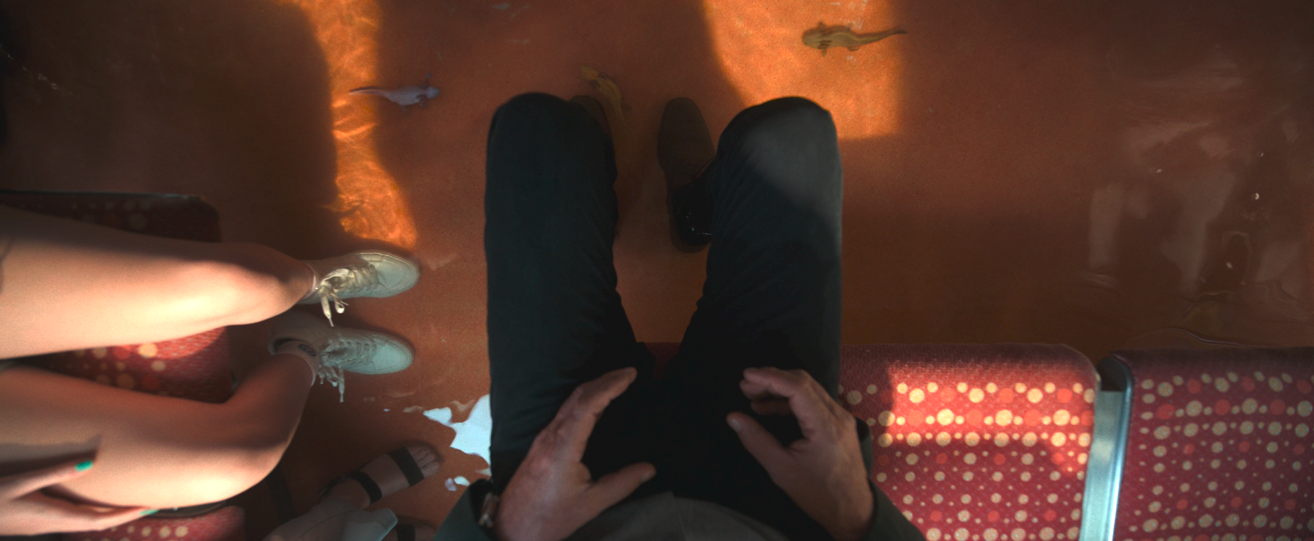 Inspiration: Stills from the movie "Bardo, False Chronicle of a Handful of Truths".
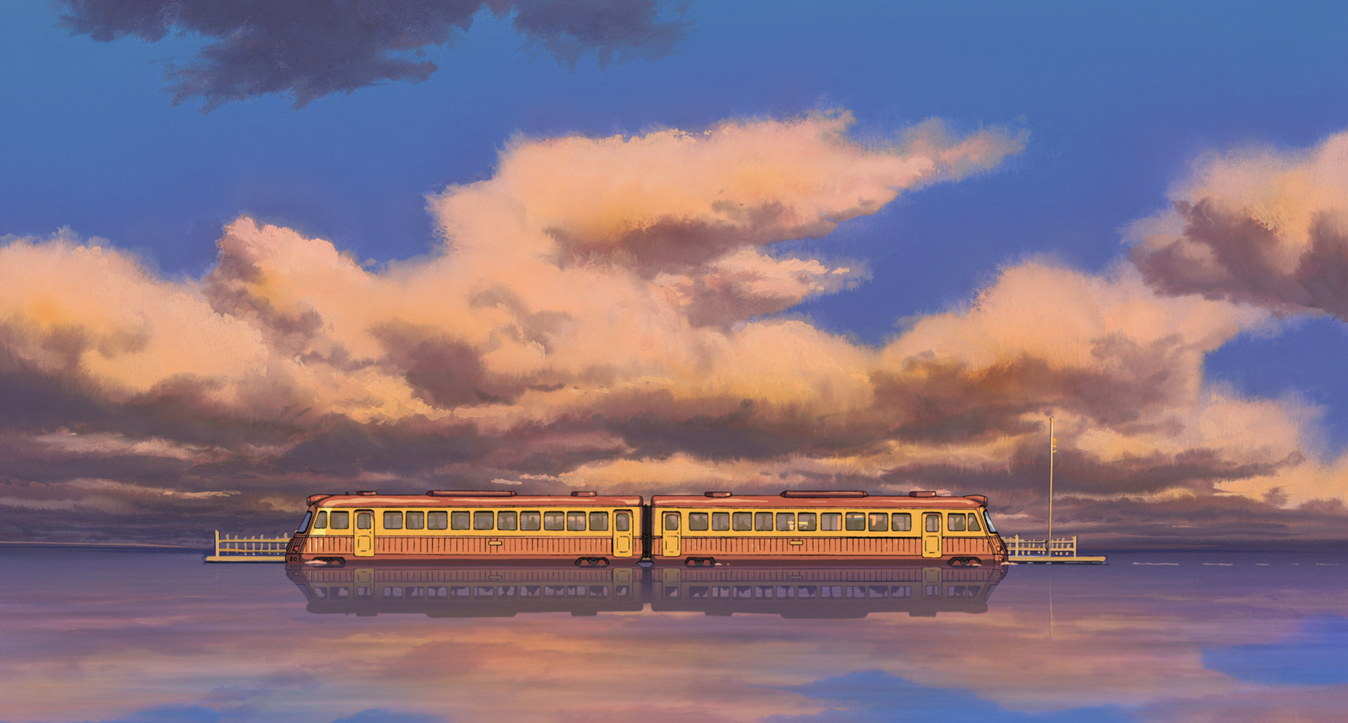 Inspiration: Stills from the movie "Spirited Away".
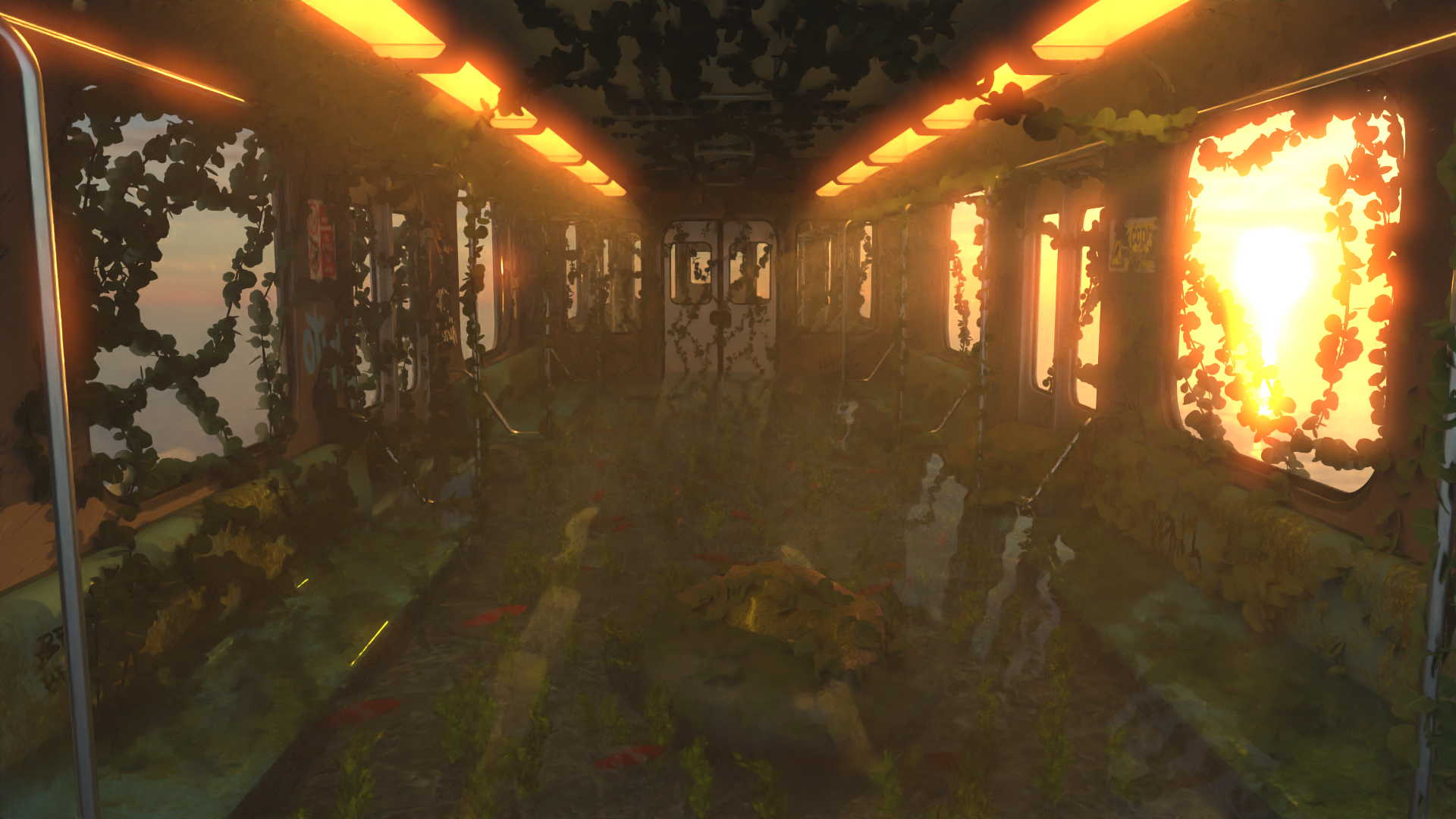
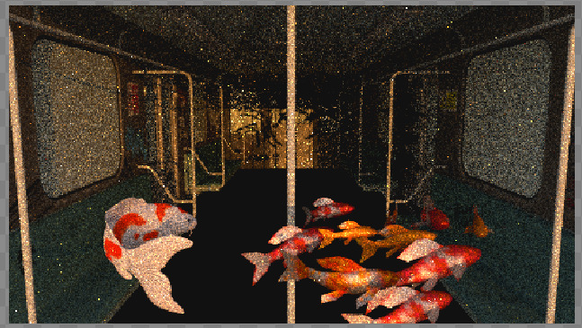
Our final image has a resolution of 1920x1080 and was rendered using 2048 samples-per-pixel and a maximum depth of 10 for path tracing. The render took 12893.91 seconds using an AMD Ryzen 7 8840HS processor and 16 Gb of RAM.
Features
Quick access list:
Alpha Masking
Alpha masking is a handy trick to simulate complex geometry cheaply. The trick is to have a special texture called "alpha mask" that tells the renderer the transparency value of each point in the mesh. The transparency is a value between 0 and 1, with 0 meaning that the point is fully transparent and would let rays pass through it even if it is part of the geometry of the object. A non-zero value will intersect the point with probability alpha (otherwise it would let the ray pass through).
One could use this trick to simulate, for example, leaves by creating a simple mesh, putting an image texture on it with the actual leaves and using an alpha mask to hide the regions between the leaves by setting their alpha values to 0.
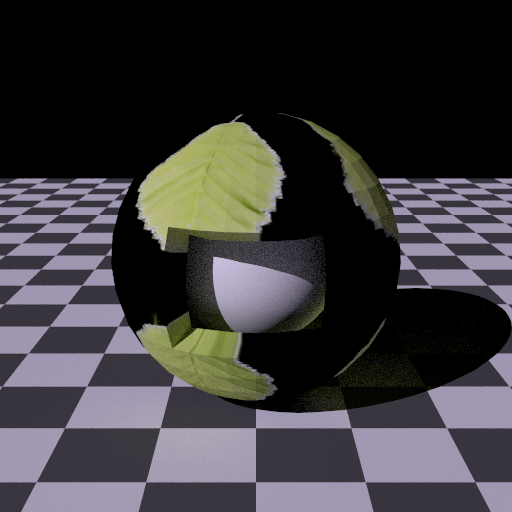
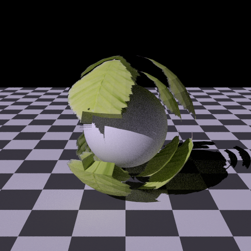
Figure 1.1: Before alpha masking (left) and after alpha masking (right).
High-level implementation summary
Files changed:
include/lightwave/instance.hppsrc/core/instance.cpp
The Instance class now has an optional m_alpha attribute, which is a Texture containing the alpha mask to be used by the instance. An alpha mask can be added to an instance by adding a Texture with the name alpha.
Having an alpha mask means that we might intersect an object multiple times before actually hitting a non-transparent surface or exiting the object.
The intersect method had to be refactored to account for multiple intersections. We used an iterative approach that repeatedly tries to intersect from the current position. If an intersection is found and the ray is allowed to go through (randomly based on alpha), then we update the current position to the intersection position and go to the next iteration.
We also had to update transmittance, which now has to treat alpha masked instances differently from regular ones. This is because in the regular case we would just call m_shape->transmittance(), but that would completely ignore the alpha mask, since m_shape does not know about it. So in the case of objects with an alpha mask, we just return a binary transmittance value based on the result of the now-refactored intersect method. This logic does not work however on volumes, but we decided that there's no reason for volumes to use alpha masks anyway.
Biggest challenge
The biggest challenge was figuring out that alpha masking has the potential to "go through" multiple intersection points of the instance. This broke the transmittance method, which took some time to fully understand because we had to go through the class hierarchy to figure out how transmittance is really computed and make sure the solution we have doesn't break anything.
Area Lights
Basic area light sampling
Area lights are lights that have a surface area and can be intersected by rays. Before, in order to get contributions from such a light, we would rely on the chance that sampleBsdf would return a ray that points to such a light. Area light sampling aids in this process by allowing us to sample a direction that points to the surface area of the light, which would yield a direct contribution of this light to our shading point.
The naive method of sampling is to uniformly sample a point on the full surface area of the underlying shape. The following render shows the difference between no area light sampling and basic area light sampling. We observe a great improvement.
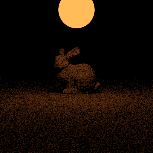
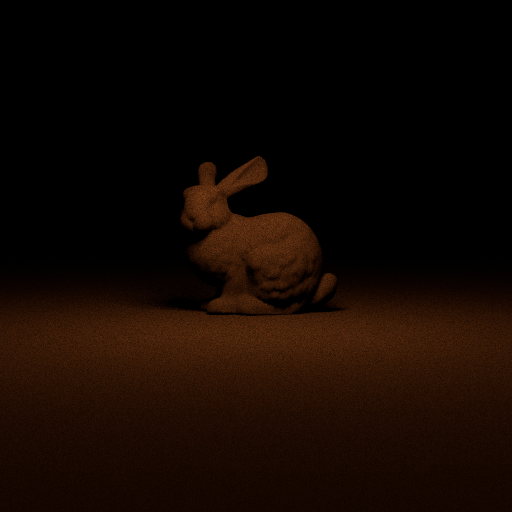
Figure 2.1: Before basic area light sampling (left) and after (right).
Improved area light sampling
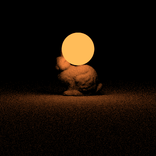
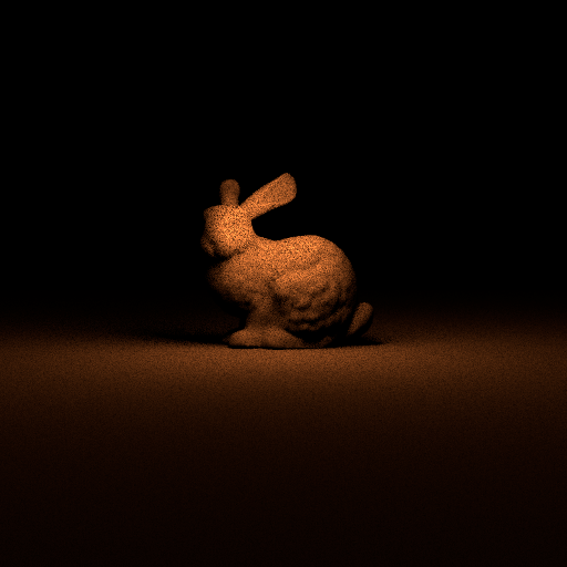
Figure 2.2: Before basic area light sampling (left) and after (right) when the light is close. Note how the bunny itself is noisier with area light sampling.
As we can see in Figure 2.2, the area light sampling is not always better than relying on chance. This is because the geometric term of the estimator is divided by the distance between the shading point and the sampled point squared. When the light is too close, the contribution value blows up, which brings us back to a noisy image.
For the sphere, this can be solved by sampling the subtended cone by the sphere. The surface of the sphere confined in the cone is the set of all visible points from the shading point. This method removes the division by the square of the distance because here we sample the solid angle instead of the surface area, which simplifies the estimator. What's more, now all the points we sample are visible to the shading point. This was not the case before, as we could sample a point on the other side of the sphere, which would yield no contribution.
A comparison is shown in Figure 2.3 and Figure 2.4.
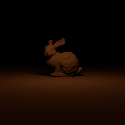
Figure 2.3: Basic area light sampling (left) and improved area light sampling (right) for a sphere.
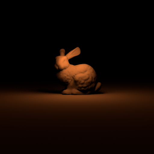
Figure 2.4: Basic area light sampling (left) and improved area light sampling (right) for a sphere when the light is close.
High-level implementation summary
Basic version
Files added:
Files changed:
src/core/instance.cppsrc/integrators/direct.cppsrc/integrators/pathtracer.cpp
The basic area light sampling required virtually no change to the integrators, although the comments had to be updated. Besides that, a new class AreaLight has been added, which has an m_shape member of type Instance, which describes the shape of the light in world space. It implements the logic of computing the light contribution of a sampled point on the surface of the underlying shape.
The Sphere::sampleArea method had to be implemented, which initially sampled the surface area of the sphere uniformly.
Improved version
Files changed:
include/lightwave/instance.hppinclude/lightwave/shape.hppsrc/core/instance.cppsrc/lights/area.cppsrc/shapes/group.cppsrc/shapes/mesh.cppsrc/shapes/rectangle.cppsrc/shapes/sphere.cpp
For the improved area light sampling, the header of the sampleArea method had to be changed to include the shading point coordinates, as this was required by Sphere::sampleArea. For the sphere, sampling is done on the subtended cone by the sphere from the shading point.
Biggest challenge
Two big challenges:
- Figuring out how to update the value of the PDF when the object is scaled. This was not very intuitive, but the solution was very elegant. In short, the PDF had to be scaled by the lenght of the cross product of the tangent and bitangent, which gives essentially a stretch factor for the local area around that point.
- Improving the sampling for sphere lights has been quite difficult to grasp as there are different coordinate systems to consider at the same time and the math is not too easy either.
Bloom
Bloom is a postprocess that creates artificial light diffusion in a certain region of the given image, it is usually used to simulate artifacts that real cameras produce, such as halation in photographic film, digital sensor saturation or the imperfect focus of real lenses. Aesthetically, it gives realism to a rendered image, and helps sell the illusion of blindingly bright lights, so it is typically used in the highlight regions of an image. Some examples are contained in Figure 3.1.
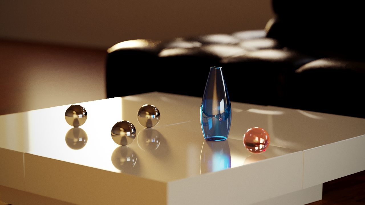
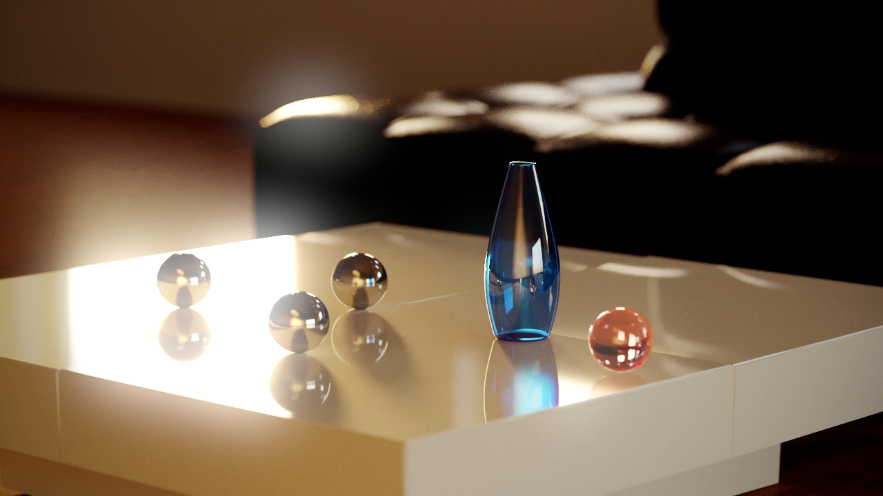
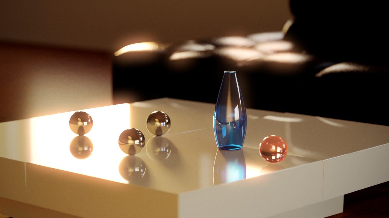
Figure 3.1: Before bloom (first), bloom with default settings (second), bloom with personalized settings to create a film-like halation effect (third).
High-level implementation summary
Files changed:
src/postprocesses/bloom.cpp
The changes for this feature are fully contained in the bloom.cpp file. The member variables are read from the scene XML to enable the customization of the effect:
m_sigma: The standard deviation of the gaussian function. Dictates the "strength" of the effect.m_size : The size of the gaussian kernels. This is calculated using m_sigma to ensure rounded bloom edges.m_threshold: The luminance threshold that determines the regions of the image where the effect will be applied.m_tint : An RGB factor to tint the blooming with a specific color for artistic purposes.
Our implementation creates bloom by taking the input image, masking a desired region to apply the effect to, in this case the pixels that exceed a certain luminance threshold, and using a 2D gaussian function as a convolution kernel. Here, we take advantage of the commutative nature of gaussians to simplify the 2D convolution into 2 passes of 1D convolution.
To do this, first the createGaussianKernel() function takes a boolean to create either a horizontal or vertical kernel, using the X and Y dimensions of the image. Then, using the applyConvolution() function, the thresholded image is blurred horizontally using the X kernel and then vertically using the Y kernel.
After both passes, the result is tinted using the user-defined factors and then simply added back to the original image to get the final "bloomed" image such as those in the examples.
Biggest challenge
The biggest challenge here was actually choosing how to implement the elements of the effect, for every stage of this process there are many different methods that yield very different results. For example, the thresholding could also be implemented with a soft & hard threshold where areas around those that meet the hard threshold can also have the effect applied to them, instead of having a hard cutoff. In a similar way, the calculation of the kernel size provided very different results,too low a kernel size diffused the light too much, producing a "dirty" image and the opposite resulted in squared bloom. Another example is the blending mode, here we use a linear dodge (additive) mode to blend the result of the convolution to the final image, but there are others like lighten, screen, overlay, etc.
In the end, we chose simplicity and ease of use, i.e. minimizing the number of options and parameters that need to be passed in the scene XML and used what provided the best looking results in our testing.
Denoising
Denoising is a special kind of postprocess that is used to remove or mitigate the sampling noise that comes naturally with the use of the stochastic sampling methods such as Monte Carlo. For this, the Intel Open Denoise library was used. This library is specifically geared towards renders that were created with ray tracing, and is based on deep learning denoising filters that were trained on a wide array of sample-per-pixel numbers to ensure consistent results. Denoising is especially useful for busy scenes, as calculating the light contributions of all possible light sources stochastically would require a great number of samples and would increase rendering time significantly. Some examples for the results produced with this postprocess can be viewed in Figure 4.1.
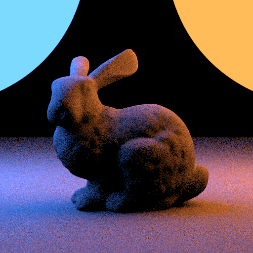
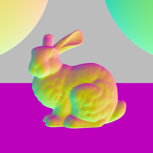
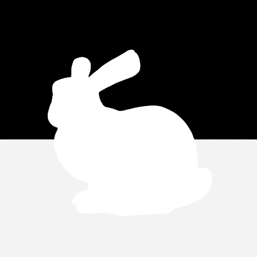
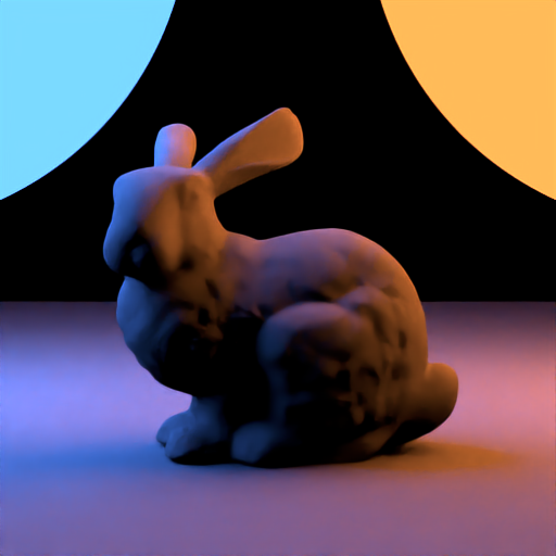
Figure 4.1: Original noisy render (first), normal image (second), albedo image (third), resulting denoised image (fourth).
High-level implementation summary
Files added:
Files changed:
include/lightwave/bsdf.hppsrc/integrators/aov.cppsrc/postprocesses/denoise.cppsrc/bsdfs/conductor.cppsrc/bsdfs/dielectric.cppsrc/bsdfs/diffuse.cppsrc/bsdfs/principled.cppsrc/bsdfs/roughconductor.cppsrc/bsdfs/hg.cpp
The Intel Open Image Denoise library was added to the project dependencies.
The denoising requires an albedo image as an input, so the AOV integrator was extended to support this feature. For this, the bsdf base class was extended with a virtual method evaluateAlbedo() and this method was implemented in all of the preexisting bsdfs to return the correct albedo.
The main denoising pipeline was implemented in denoise.cpp where we initialize the denoising device, create the denoising filter, allocate memory for the buffers corresponding to the 3 input images and finally apply the filter and read the output image.
Biggest challenge
The biggest challenge we faced for this feature was understanding the way in which the denoising pipeline worked and how to implement it into our codebase, we originally used a lot of unnecessary computation and memory which we later optimized once we got the correct understanding of how the buffers were used to input and output the images.
Mix Shader BSDF
This is not a feature mentioned in the project features list, but we decided to implement a new type of BSDF which is supposed to simulate the "Mix Shader" node of Blender. The idea is to mix two different BSDFs based on a weight factor (in other words, a weighted average). This allows us to mix different materials to obtain effects such as adding moss on a rocky surface.
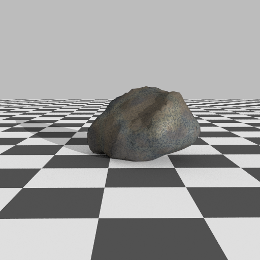
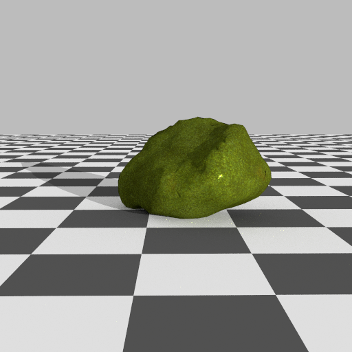
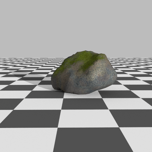
Figure 5.1: A principled BSDF that gives a metallic look (first), a principled BSDF that gives a mossy look (second), and a mix BSDF mixing the two principled BSDFs into a single one based on a weight texture (third).
High-level implementation summary
Files added:
We can now declare BSDFs of type mix. A mix BSDFs requires two child BSDFs first and second and a texture weight to weight them by.
The Mix class implements Bsdf. BSDF evaluation is done by performing a weighted average over the evaluation results of the two child BSDFs. BSDF sampling is currently done by probabilistically sampling one BSDF or the other (over time, this averages out to the true mean).
Biggest challenge
The biggest challenge has been figuring out how to do the sampling. The best way to do sampling would be to sample a direction wi probabilistically according to the current weight, compute the pdf value of this direction for **both** BSDFs and then return a weighted average of the evaluations of the BSDFs based on the PDFs and the weight factor. Unfortunately, the way the framework is constructed, BsdfSample and BsdfEval do not have a pdf field, so we resorted to the simpler stochastic method for sampling.
Normal Mapping
Normal mapping helps in creating more realistic details without requiring a complex mesh. The normal map is a texture which stores the direction of the normal for a given uv coordinate.
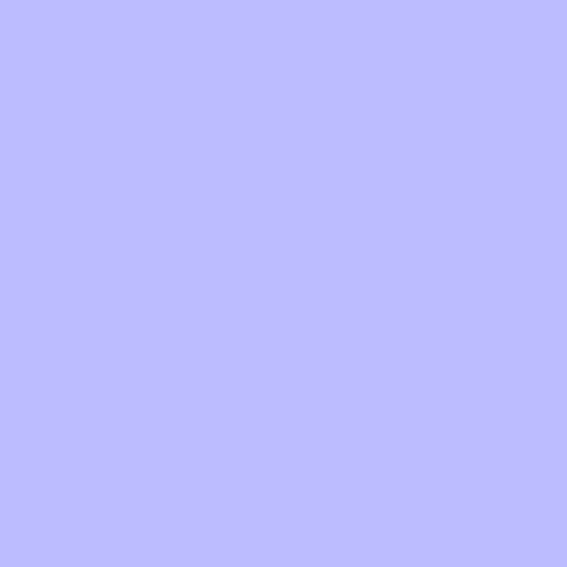
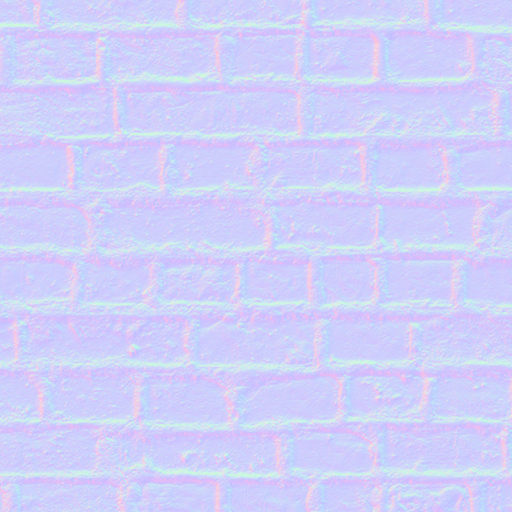
Figure 6.1: Normals before normal mapping (left) and after normal mapping (right).
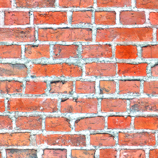
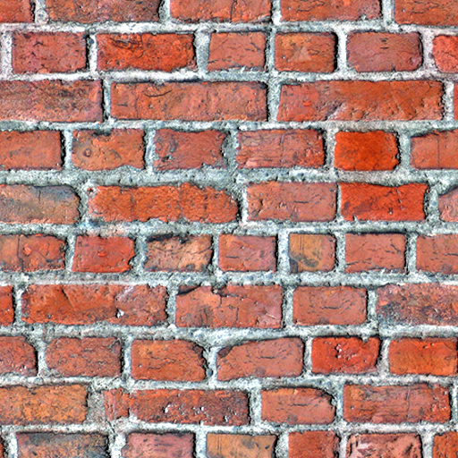
Figure 6.2: An example that shows a normal map in action. Shading before normal mapping (left) and after normal mapping (right).
High-level implementation summary
Files changed:
include/lightwave/instance.hppsrc/core/instance.cpp
The Instance class now has an optional m_normal attribute, which is a Texture containing the normal map to be used by the instance. A normal map can be added to an instance by adding a Texture with the name normal. If an instance does not have a normal map, it uses the normals provided by the intersection code.
Biggest challenge
The biggest challenge was creating a proper test scene as we were not 100% comfortable with the XML format of the scene.
Render
We started by drawing a sketch of the scene and brainstorming possible ideas for the composition and we settled on this one:
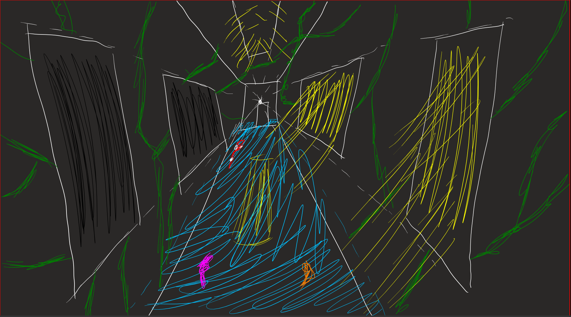
During the creation of the scene we experimnted with many assets, textures and layouts, the first major decision was choosing a mesh for the fish in the scene. We had many different options but landed on two main options, the first was much more detailed but required us to repaint the texture in different colors and rig the fish in order to have it positioned in different ways, instead of copying the same fish in the same position many times. This proved to be more time consuming than necessary so we opted for an asset that already contained a school of Koi fish with different patterns, colors an positions, which we could simply scatter and duplicate around the scene. To simulate water, we used a plane with a noise texture as a normal map that creates the illusion of ripples in the water and gave it a dielectric BSDF as a way to create the reflections on its surface while still allowing us to see into it.
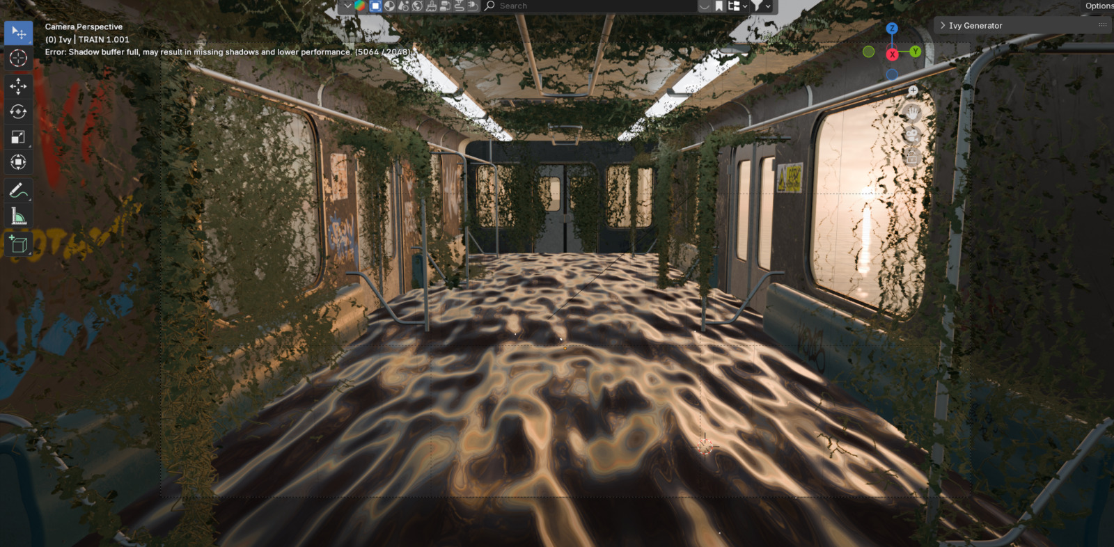
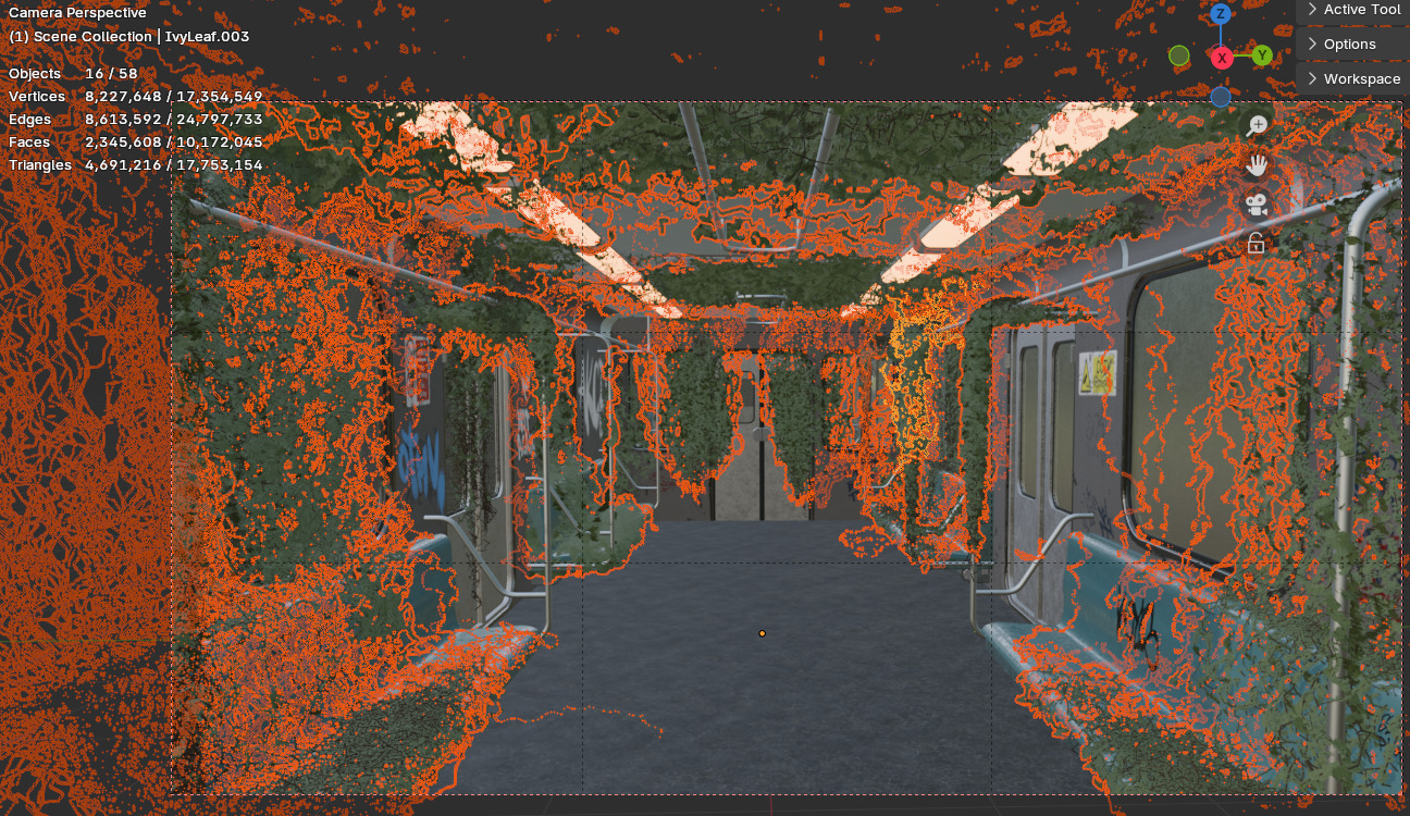
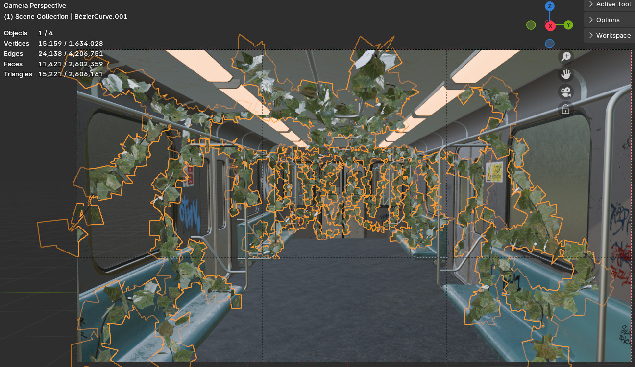
Next we experimented with many different types of foliage. The first option we considered was a preexisting asset of vines in an abandoned building, but these were hard to repurpose and stage in our specific scene. Then we experimented with a blender add-on called IvyGen that creates procedurally generated Ivy, and this was how we set up our scene for the majority of the process, but it had two major problems. The first was that the plugin only allows you to control the starting point of an Ivy and some parameters about how it is generated, but ultimately abstracts away too much control and it was frustrating having to continuously regenerate until we got a result we were happy with. The second big problem with this methos, was that it created an enormous amount of geometry, and even though it was simple geometry, the numbers added up fast and all the benefits of using alpha masking eventually were overshadowed by having millions of leaves and branches (which very frequently managed to crash our computers). The solution for this was creating a custom geometry node system that extruded a simple tubular vine and instanced simple planes which, using alpha masking became the leaves. This not only meant that the amount of vertices and triangles was dramatically reduced, but it also meant that we could draw the vines on surfaces and decide precisely where we wanted them to go.
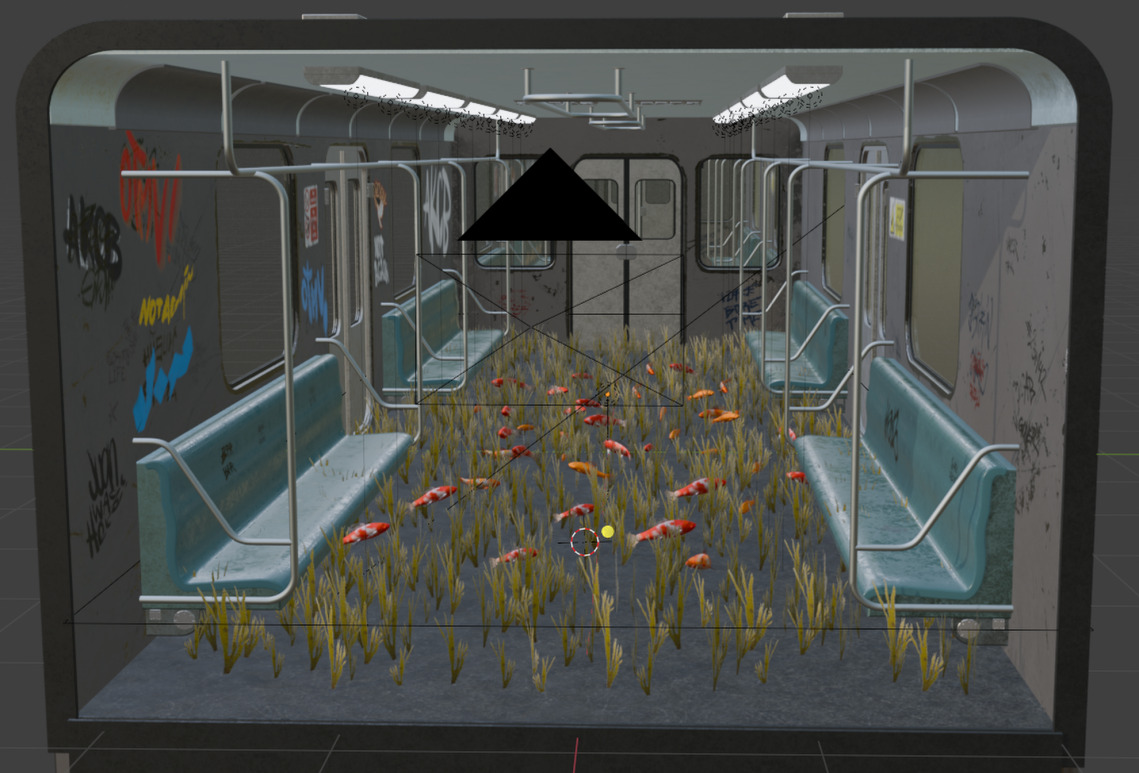
The next thing we wanted to add was seaweed and for this we placed a plane aligned with the subway floor and used a particle system to create many copies of a single seaweed with variations in placing, size and orientation. We created two version for this. One in which each seaweed was just a plane with an alpha mask, and another where each one was a mesh. The consideration here was the performance, but we managed to decimate the geometry of the mesh down to a couple thousand triangles, so we decided the small hit in preformance was definitely worth the bump up in quality.
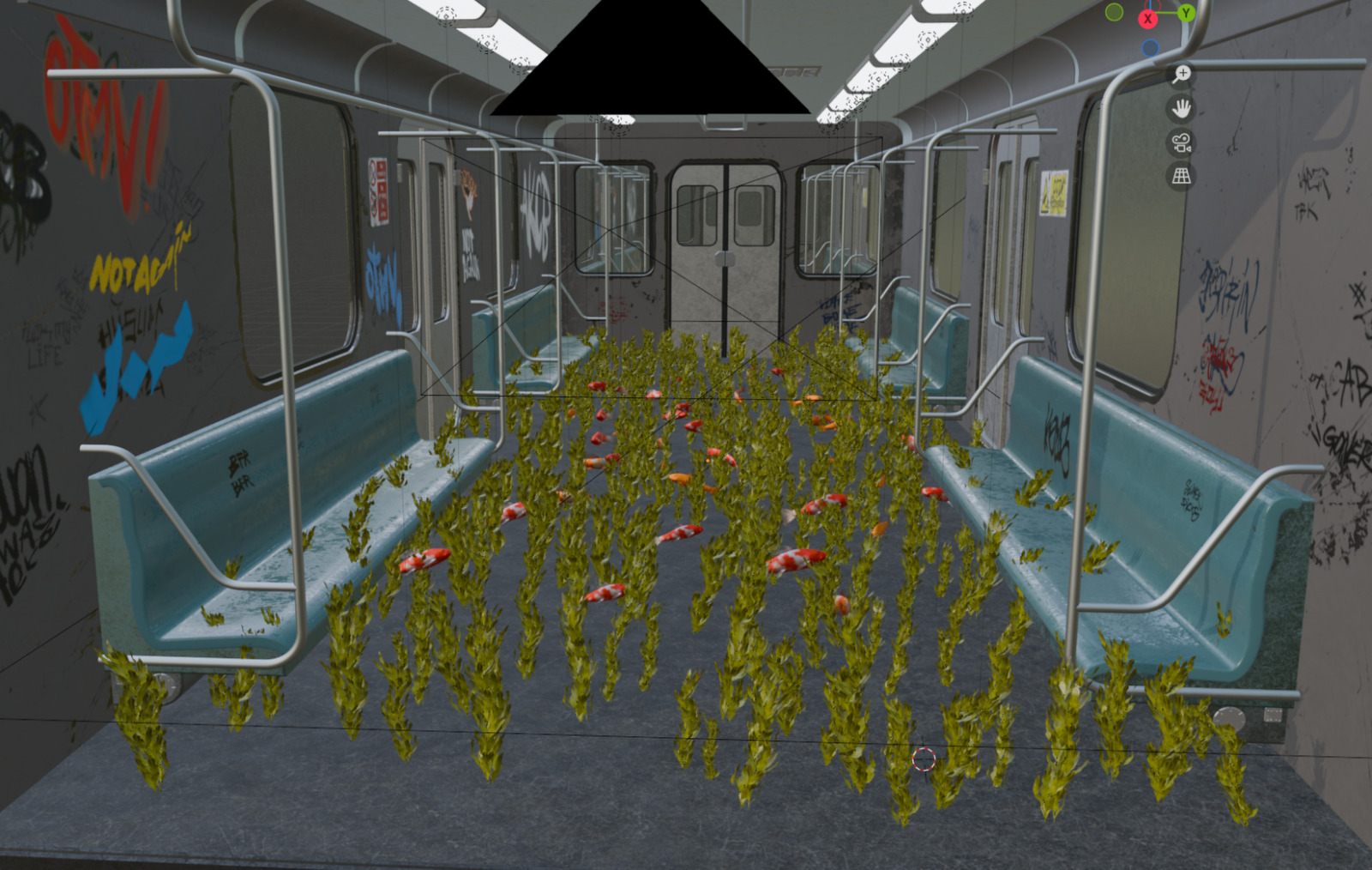
After getting a solid layout of the scene, we went on with experimenting with the different parameters of the rendering process. After many attempts we found a satisfying solution which can be observed in the background and here: