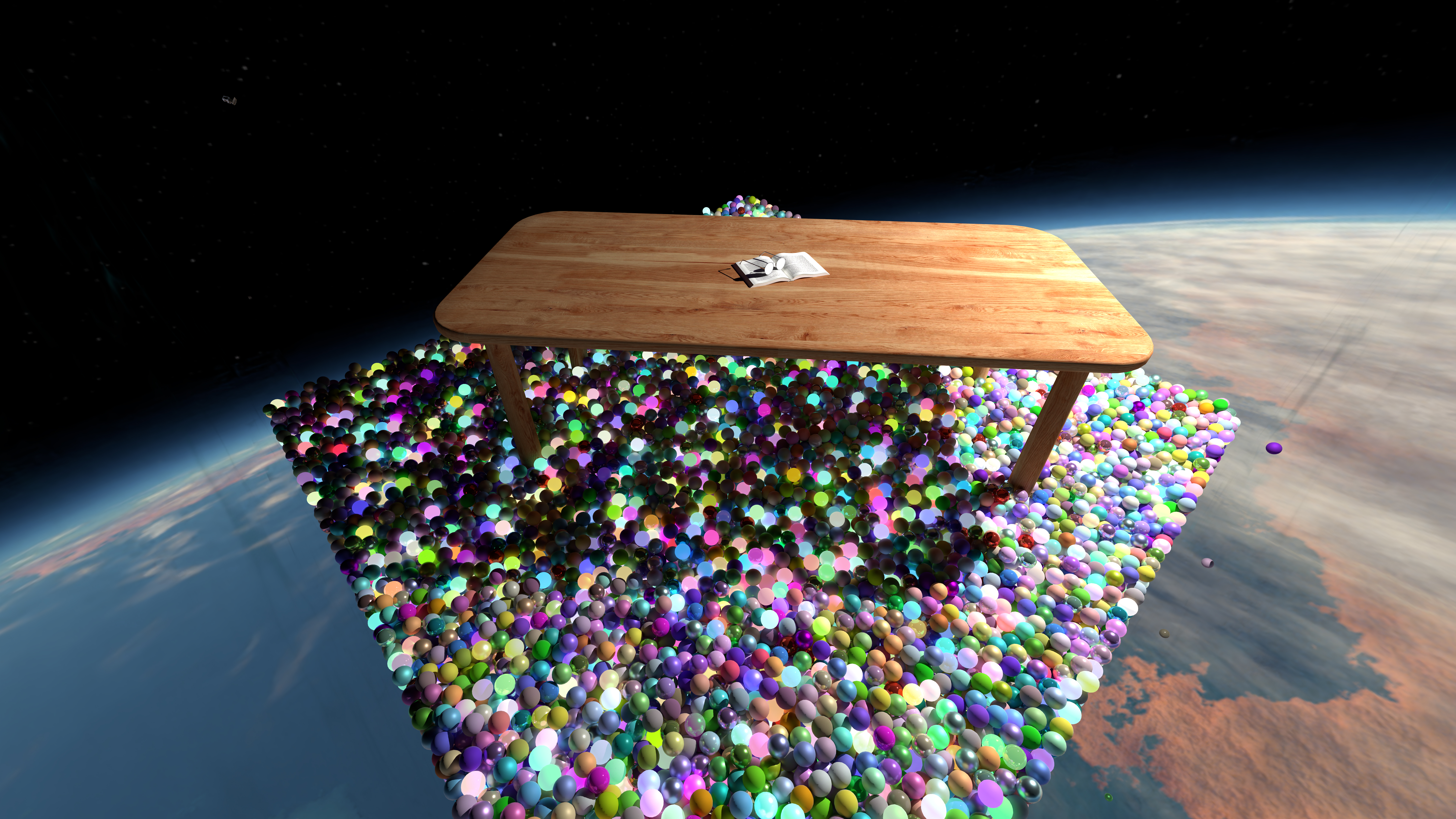
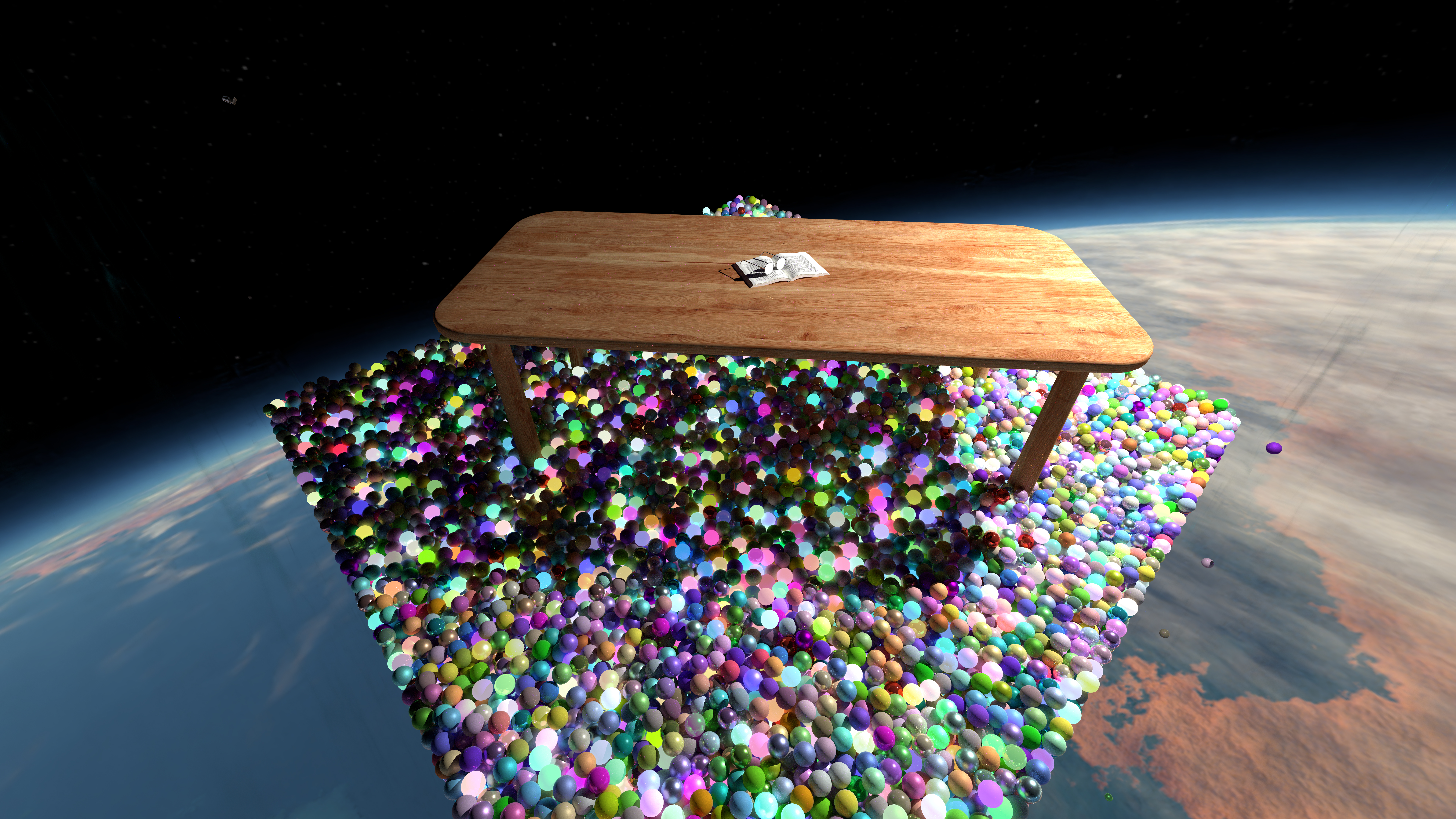
The main idea behind this scene is the growing fight between elegance in simplicity, and the chaos and disorder
of our increasingly digitalized lives. The many spheres with their bright colors stand in stark contrast to the
elegance and "quiet simplicity" on a minimalistic wooden table. The viewer is presented with a
choice: either giving their attention to the bright, colorful sea of impressions or to appreciate the quiet
simplicity at the center of the scene.
Social media is in many ways similar to the "distracting" background of the scene. Everything is bright,
colorful and loud, always fighting for our attention. Things as simple as reading a book can be considered
quite the opposite, and yet their "boringness" can serve as a calming escape from this digital fight for our
attention we find ourselves in every day. At the same time, we feel distanced, far away from reality
and our loved ones.
The scene itself consists of roughly 11.000 balls, with 100 randomly generated bsdfs and emissions assigned to
them. The balls were created in Blender, given a physics-simulation to nicely distribute them and then
exported (frame 112 to be exact). The textures and emissions were not actually created in Blender (more on that
later). The two walls closest to the camera also have a faint plasma texture applied to them, which uses
alpha mapping.
Third Party Asset Credits
General Notes
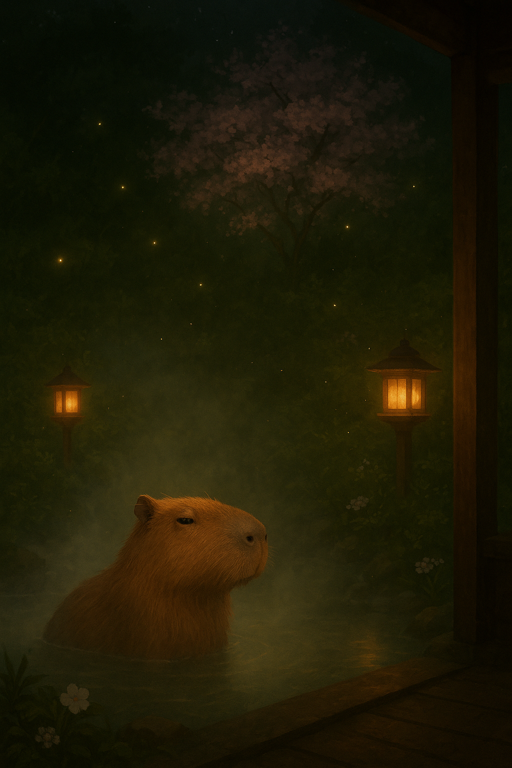
Our final scene is in fact not the scene we originally wanted to create for the rendering competition. The very
first scene that we had in mind was a kind of "Capybara Onsen", loosely inspired by its real life counterpart. The
scene would take place at night, with moonlight reflecting in the water, fog hovering above the water and some
fireflies in the air. Using ChatGPT, we quickly generated the following concept image:
We knew that we would need both heterogeneous volumes as well as hair for this scene, which we knew would likely
not be easy. An additional problem that we soon discovered was the surprising lack of good-looking capybara
models (at least for less than 150€). Therefore we soon switched to a scene still involving water and nice fog,
but without the hair (and capybaras).
As the project deadline grew closer however, we were not entirely certain whether we would
actually be able to implement advanced and heterogeneous volumes in time, which were necessary for our scene.
This resulted in us
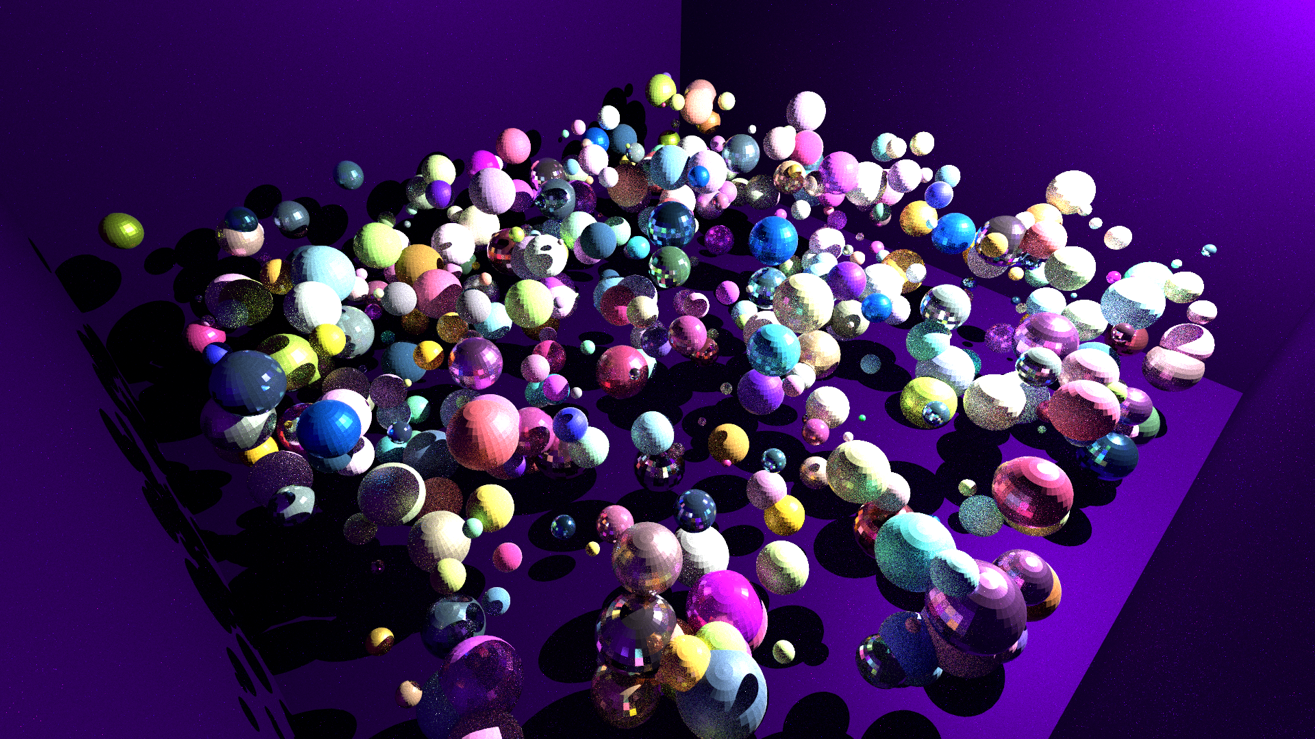
effectively building a second final scene, initially only depicting a large number of spheres in a mostly empty
room.
Early version of our final scene:
We soon started liking this scene so much that we decided to use it as our final scene. We did end up also
implementing advanced volumes, with the following being our original submission, expanding on the idea and
eventually reaching our final scene.
Early version of what was originally going to be our final submission.
While building our scene, the thing we struggled with most was finding suitable assets that the blender-exporter
could actually export, as well as including OpenVDB into our renderer, in order to allow for rendering advanced
volumes. OpenVDB provides an efficient grid representation, and is used by big production renderers like
Blender,
Houdini and Maya.
Almost all good-looking models online used at least one of Blenders ShaderNodeMix,
ShaderNodeBump or ShaderNodeAdd shader nodes, as well as those generating procedural
textures, which were not supported by the blender exporter. Many assets also use procedurally generated
textures,
which were also not implemented. For most of our assets we had to resort to manually editing the
shader graphs
of these materials, removing the unsupported nodes and playing around with the remaining nodes until the result
looked acceptable, before finally being able to export the asset. In addition, many of the example scenes for
the
individual features were mostly tweaked in the corresponding xml-files.
In particular, we created a couple of python scripts, which operate directly on the lightwave xml files. This is
further complicated by the fact, that these files strictly speaking do not adhere to the xml standard, since
they
have more than one root element. Most python xml-libraries do not cope with this well and throw an error, so we
had to resort to a smaller xml library (python-lxml)which allowed us to tell it to recover from any
parsing errors.
One of these scripts for example is used to apply an arbitrary amount of randomly generated principled bsdfs to
some shapes in the xml file, which is how we achieved the large amount of unique spheres in our table scene.
The other script was only used early on to create the spheres, before we found out how to better model and
physically simulate the spheres in Blender.
Alpha Masking
Alpha masking refers to adding an (optional) texture to objects in a scene, which describes how translucent
the surface of this object is.
Alpha masking is implemented by adding a new alpha-texture to the Instance class. We then adapt
Instance::intersect and Instance::transmittance to use this texture. The scalar value
of the texture at the intersected position determines the probability of a hit actually being counted or being
ignored.
One question we were not immediately sure about was whether or not we should also sample the alpha texture on
internal intersections, meaning whether or not it's possible for a ray to be let through (into) a shape but not
out on the other side. We temporarily had a bug that caused the alpha mask of one of the two faces to be
inverted, while the other one worked as expected. This was caused by a flipped less than sign in the code.
Having fixed this, alpha masking now works as expected.
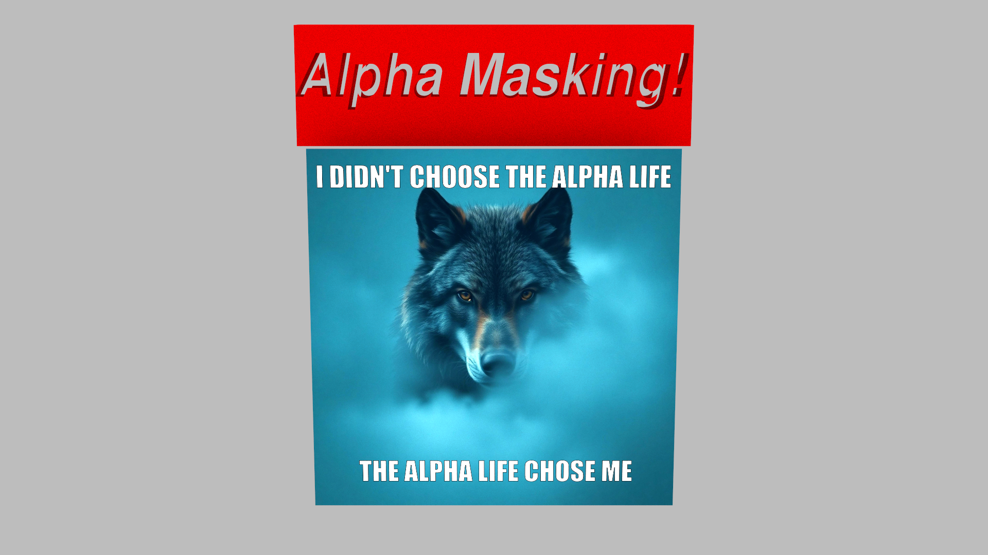
Example image that uses alpha masking in order to mask text (the headline) out of a cuboid:
Denoising
The process of denoising involves taking an image which has some noise in it, and outputting an image with as
much of this noise removed as possible. Depending on which denoiser is used, auxiliary data like albedos,
normals or other data can be provided as well in order to improve the result of the denoised image.
For denoising, we make use of Intel open image Denoise (OIDN),
which is an open-source framework for denoising ray traced images, with both CPU and GPU support. We implemented
denoising as a post-processer inside src/postprocesses/denoising.cpp with no modifications to any
other files. This turned out to be rather straightforward, as Intel provides a bit of C++ example code on how to
use OIDN. We start by creating an OIDN device and allocating appropriately sized buffers for all pixels of
output images. Optionally, we also create the buffers for albedo and normal images, which can be passed to OIDN
to further increase the quality of the denoised image. We then create an OIDN filter, to which we pass these
buffers, followed by populating the buffers with the individual images data and then executing the filter and
saving the output image.
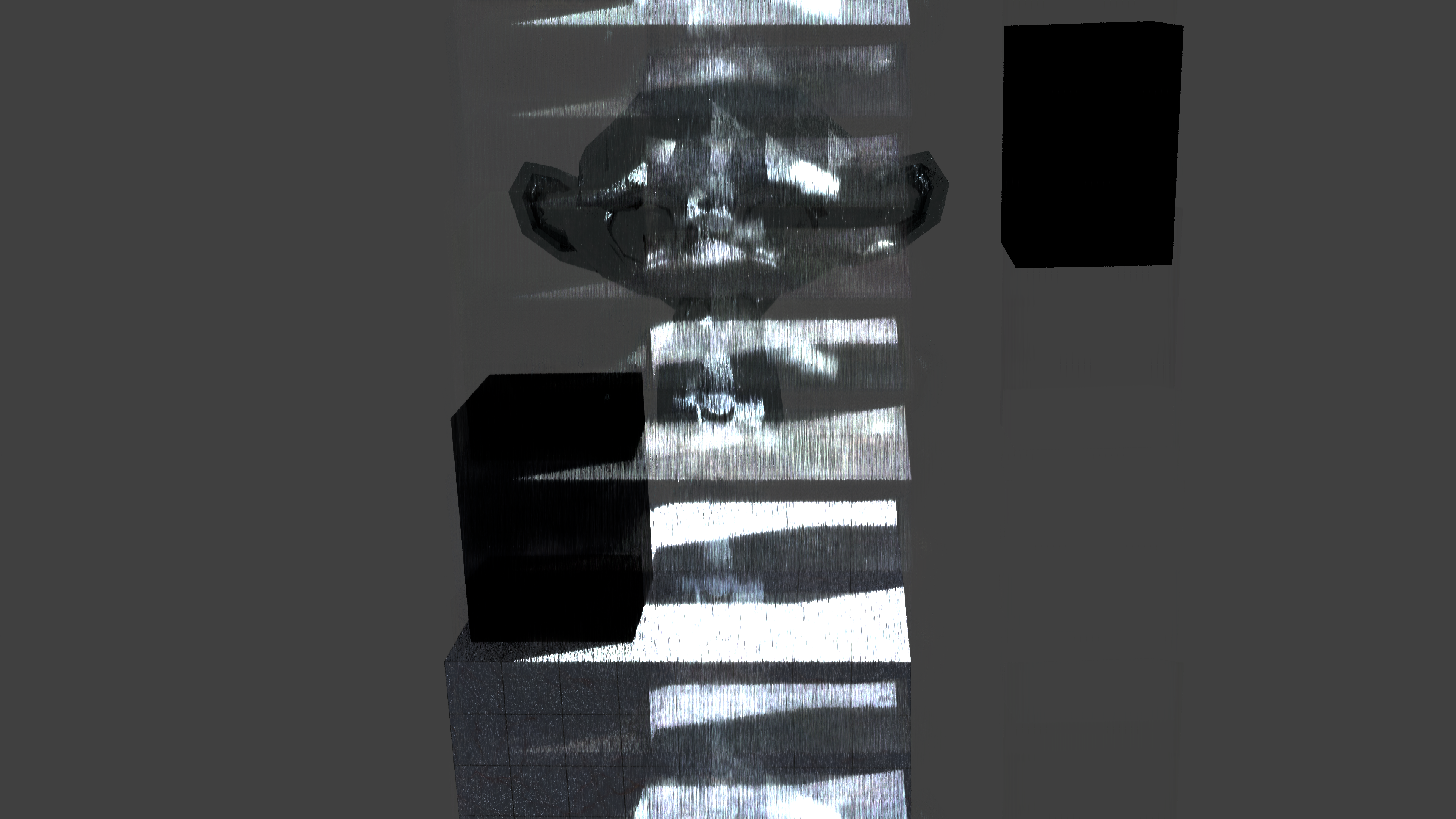
Initially, we had an interesting bug, which caused the output image to contain "smears" and ghostly
outlines of the objects in the scene at wrong positions in the denoised image.
This was caused by a typo in the for loop that loaded the image data into the buffers, since we were incorrectly
iterating over the image column by column, while OIDN expects the data to be in row-major order. We initially
thought that we were using OIDN incorrectly or that we were using the wrong datatype for the buffers. Fixing
this
gave us nicely denoised images, with even input images that only use a single sample per pixel looking
surprisingly sharp in the final result, especially when supplied with auxiliary albedos and normals.
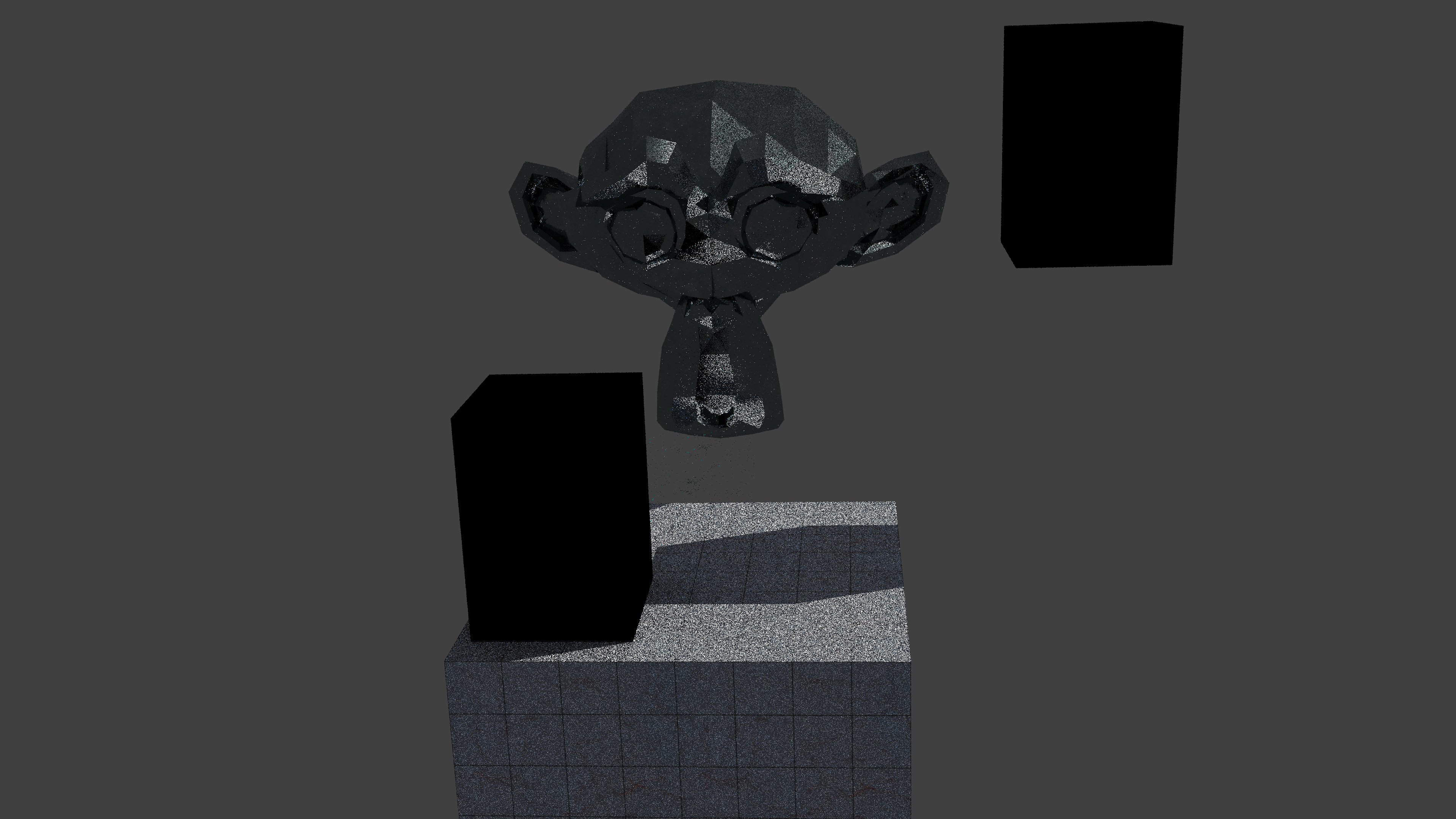
Example input image using a BSDF with only a single sample per pixel:
The Denoised image:
Normal Mapping
Normal mapping involves giving objects an optional normal texture, which is subsequently used to modify the
normal vector of the object's points according to this texture. This provides a computationally inexpensive way
to add surface details to the objects in a scene.
This feature was relatively straightforward to implement and did not cause us any bigger problems.
As suggested in the provided description of the feature, we added an optional texture to the
Instance class and changed our Instance::intersect method to evaluate and use the
normals from the texture (in case one was provided). Having implemented normal mapping allows us to for example
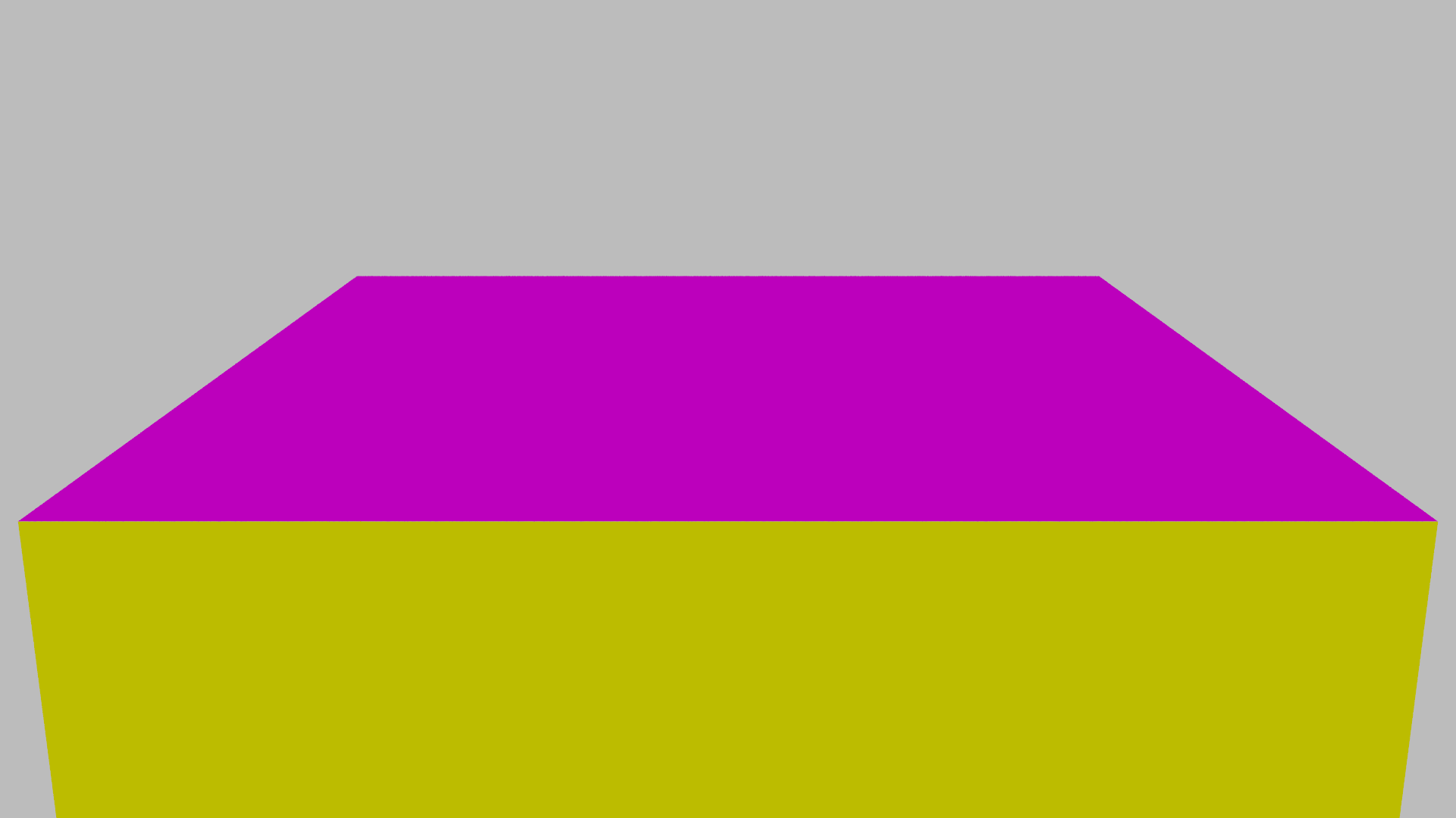
add details like grooves in a texture, without needing to change many individual textures. Image of a AOV integrator rendering normals for a simple cube mesh:
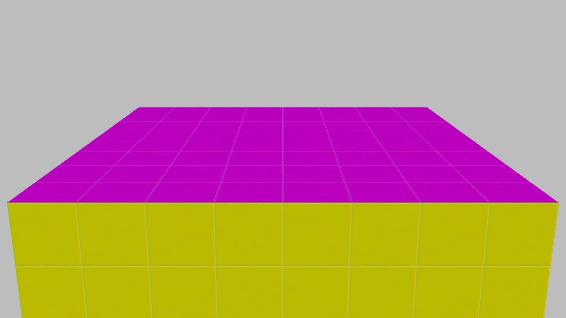
The same cube with a grid-like normal texture (same as in the denoising example) applied (and the same AOV
integrator):
Advanced Volumes
Advanced volumes are volumes that are not limited to grayscale attenuation and that can have an emission.
Implementing these additional options was non-trivial, since they disable many simplifications in the rendering
equation
that made the implementation of simple volumes rather easy. Of course, the Volume class had to be
extended
to include a Color for density instead of a float, and additionally absorption and
scatter values.
The average density is still used for importance sampling, which means that the pdf must now be included in the
render calculation, since
it no longer cancels out with the transmittance. This is partially implemented in
Volume::transmittance, which
divides the calculated transmittance by , but only if not evaluating shadow rays (for which an additional parameter had to be added to
Shape::transmittance). This change is sufficient for rays that either pass through the volume
or hit an object inside of the volume. If however the ray hits inside of the volume, leading to a volume
scattering or absorption event, the calculated values have to
be multiplied with the scattering or absorption coefficients and divided by 𝜎, which is the normalization factor of the sampling pdf. This was implemented by saving these three
values in
Intersection and using them in the Pathtracer together with the transmittance. If a closer
intersection is found, the values are
overwritten, removing the need to handle in-volume object hits differently from behind-volume object hits.
The difficulty of this feature was twofold: One part was to understand the implications of the extended volume
parameters, the other part was to find the remnants of a failed
volume implementation in math.hpp which were messing up the computations.
Volume Test From Practical Assignment 4
Color(1,1,1) - Phase Function Albedo as the Density Vector
Density Vector From the Previous Image Split Equally into Scatter and Absorption, Emission(1,0.5,0.5) added
Heterogeneous Volumes (INCOMPLETE)
The density of heterogeneous volumes varies throughout their bounding box, allowing for more realistic fog,
fluids and more.
The File Format and Considerations
To implement heterogeneous volumes, we opted for the OpenVDB file format, since it is widely used
and, most importantly, used by Blender
for its fluid/smoke simulation caches, allowing direct exporting from a scene. To read these files, we used
nanoVDB, a library optimized for using
OpenVDB grids in rendering. Before that, however, we needed to consider coordinate spaces.
Coordinate Hell
OpenVDB grids are stored in their own local voxel space, where coordinates are integers. Values between voxels
can
be interpolated using
different methods. An OpenVDB file can optionally store a world transform, which maps the local voxel space to a
variable world space. In Blender for fluid simulations,
this world space is not the Blender world space, though it has the same scale. Instead, its origin is aligned to
a
corner of the fluid domain's bounding shape, namely the corner
corresponding to the minimum of the shape's bounding box when viewed in Lightwave object space (in Blender,
fluid
simulations can only be bounded by rectangular cuboids). To obtain a transformation
between OpenVDB world space and Lightwave world space, a routine had to be added in
Instance::Instance(): It transforms the bounding shape back to
Lightwave world space, then constructs the transformation that axis-aligns the bounding shape and transforms its
bbox::min() to world origin. This transform
can then be used as the transform between volume and world space.
Compilation Hell
The next challenge was to integrate nanoVDB and OpenVDB (both are required, since nanoVDB cannot read OpenVDB
files) into the project. Initially, this was easily done, by cloning
the shared repository and including it using include_subdirectories(). This led to errors at link
time, since both nanoVDB and OpenVDB have to be built separately.
Attempts to include them in the build process with ExternalProject were unsuccessful, as was
installing them as system-wide libraries. This was due to the fact
that, as referenced in this
Github
issue, OpenVDB inadequately provides
a find module (which contains rules on how to find library files) instead of a config.cmake (which contains the
exact locations of library files), which in turn led to CMAKE finding our
OpenVDB while building, but the OpenVDB installed as a Blender dependency while linking. This was ultimately
solved by rebuilding the system package with NanoVDB support.
Volume Tracing
The next challenge was the actual implementation of volume path tracing. We opted for a combination of ray
marching and delta tracking.
Ray marching intersects a volume by taking equidistant steps on the ray between tNear and
tFar (i.e. entry and exit distance) of the volume's bounding box and stopping when a
(per intersect call) randomly chosen transmittance threshold is reached or reporting no hit if it is not
reached.
Delta Tracking is, in essence, ray marching with a semi-random step size based on the maximal density of the
volume. Unlike ray marching, this always converges to
the mathematically accurate solution and is potentially faster, if either the volume density is rather uniform,
or
the volume is efficiently split into density areas.
For information on these algorithms, we found this document by Steve
Marschner, Cornell University to be very helpful.
While delta tracking is efficient for sampling intersections, it cannot be used for transmittance calculation,
which is necessary for both next event estimation and non-grayscale densities. Therefore, we
use ray marching with an adjustable subdivision count for HeteroVolume::transmittance().
Unfortunately, we were not able to finish the implementation of this final step in time. While
all functions are implemented, they likely contain bugs, and the volumes do not interact with light as intended.
See the images below for reference.
The smoke volume was emitted from the central sphere in a smoke simulation. Its bounding box appears correctly
...(In the EXR, the sphere's bounding boxes are also visible, this was lost in the PNG)
... but the volume itself is invisible on the render
Halton Sampler
The idea of low-discrepancy sampling is to have points that are somewhat randomly, but evenly distributed over
some range.
We also quickly gave implementing the Halton Sampler a try, since it didn't seem like too much work from
reading the PBR-book. The overall concept of how the point distribution works, didn't seem that complicated
either and we quickly threw together a simple implementation in samplers/halton.cpp. After some
initial confusion about how we should go about implementing the seed functions of our sampler, we arrived at
something that seems like it is almost working. Unfortunately, it does not seem like our sampler delivers
noticeably better results when compared to the independent sampler, providing a little bit more noise if
anything at all.
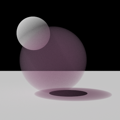
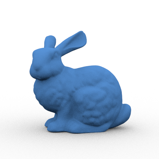
Image rendered by the independent sampler
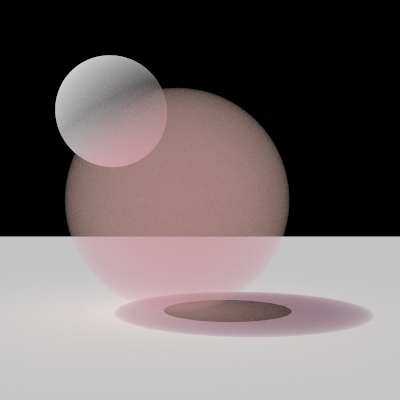
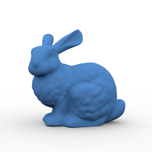
Image with same amount of samples, rendered using our Halton sampler